Numerical Methods

Numerical methods are an indispensable part of today's engineering toolkit. We shall focus on two popular techniques used to solve electromagnetic problems. (There are many other approaches and the advanced reader is referred to books like Numerical Techniques in Electromagnetics, by M. N. O. Sadiku.)

1. Finite Difference Time Domain (FDTD) is a popular method used in time varying problems and solves Maxwell's equations by alternatively solving for the electric and magnetic fields at each time step.
2. Relaxation Method provides an iterative solution to Laplace's or Poisson's equation in two dimensions. Given the boundary potential, the potential at all lattice points on a 2-D grid is obtained by substituting at each point a weighted average of the values at its nearest neighbours and repeating the procedure till convergence is achieved.

Most numerical methods will converge to the same solution. However, the final accuracy of the final result depends on a judicious choice of boundary conditions. The boundary conditions are themselves not always obvious when one is faced with an engineering challenge.

Dirchlet and Neumann boundary conditions

Yee's FDTD algorithm

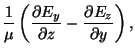
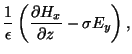
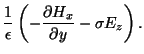
Assume a 2-D rectangular cross-section in the y-z plane. The outer surface of the rectangle is excited by a sinusoidal $\vec{H} = H_0\cos(\omega t) \hat{x}$ field. We seek the electric and magnetic fields in the interior of the rectangle. With the magnetic field always perpendicular to the rectangle, the only components of the electric field will be in the y-z plane. Expanding Maxwell's equations we get,

$$\frac{\partial H_x}{\partial t} = \frac{1}{\mu}\left(\frac{\partial E_y}{\partial z} - \frac{\partial E_z}{\partial y}\right),$$

$$\frac{\partial E_y}{\partial t} = \frac{1}{\epsilon}\left(\frac{\partial H_x} {\partial z} - \sigma E_y\right),$$

$$\mathrm{and}\;\;\; \frac{\partial E_z}{\partial t} = \frac{1}{\epsilon}\left(-\frac{\partial H_x} {\partial y} - \sigma E_z\right).$$ (18)

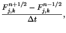
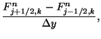
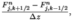
The time and space derivatives at any location $(y,z) = (j,k)$ at the time step $t = n$ can be further expanded as

$$\frac{\partial F^n_{j,k}}{\partial t} = \frac{F^{n+1/2}_{j,k} - F^{n-1/2}_{j,k}}{\Delta t},$$ (19)

$$\frac{\partial F^n_{j,k}}{\partial y} = \frac{F^n_{j+1/2,k} - F^n_{j-1/2,k}}{\Delta y},$$ (20)

$$\mathrm{and}\;\;\frac{\partial F^n_{j,k}}{\partial z} = \frac{F^n_{j,k+1/2} - F^n_{j,k-1/2}}{\Delta z},$$ (21)

where $F$ is either the electric or magnetic field component of interest. The equations for $E^{n+1/2}_y$ and $E^{n+1/2}_z$ will also include the loss terms $\sigma E^n_y$ and $\sigma E^n_z$ respectively. The implicit FDTD method, which is inherently stable, uses

$$E^n = \frac{1}{2}\left[E^{n+1/2}+E^{n-1/2}\right]$$ (22)

which upon substitution in (20) will yield an expression suitable for forward time stepping.

Figure 3: Positions of the field components using Yee's lattice.

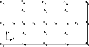An efficient implementation, by Yee, calculates H at $t=0\ldots n$ at the integer locations (j,k) whereas E is calculated at $t=1/2 \ldots n+1/2$ and at half-integer locations i.e. displaced from the H-nodes by half a cell, as shown in Fig 3. In this problem, Yee's algorithm would execute as follows

1. Start at $n=0$ and set E to zero at all interior points.
2. Initialize H on the nodes at the boundary and set to zero elsewhere.
3. Calculate $E_y$ and $E_z$ at the half-cell locations at $t = n+1/2$.
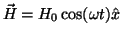
4. Set $n=n+1$ and calculate $H_x$ at the nodes. $H_x$ at the boundary is determined by the sinusoidal excitation $H_0(t)$ on the boundary.
5. Calculate the nodal average value $B_x = \mu \Sigma_{j,k} H_x$ at this time step.
6. Check for steady-state or convergence, else go to step 3.

A plot of $B_x$ versus $H_x$ will yield the hysteresis curve for this case.

Accuracy and stability of the FDTD scheme
Accuracy is often traded-off against speed of computation. Reasonable accuracy is ensured when the spatial increment $\delta = \mathrm{min}(\Delta x,\;\Delta y,\;\Delta z)$ is one-tenth the wavelength of the excitation. Stability of the FDTD scheme is ensured by demanding that the time increment satisfy

$$u_\mathrm{max}\Delta t \leq \left[\frac{1}{\Delta x^2}+\frac{1}{\Delta y^2}+ \frac{1}{\Delta z^2}\right]^{-1/2},$$ (23)

where $u_\mathrm{max} \approx c/ \sqrt{\epsilon_r}$ is the maximum phase velocity in the model.

Iterative Relaxation

Assume a uniform grid in two dimensions. The simplest method of estimating the potential, given boundary conditions, is by replacing the potential at each point by the average of its neighbours and repeating this process until the change in the potential at all points becomes arbitrarily small. In mathematical terms, this would correspond to saying that the potential $\Psi_0$ at the origin is

$$\Psi_0 \approx \frac{1}{4}(\Psi_N + \Psi_S + \Psi_E + \Psi_W),$$ (24)

where the subscripts represent the 4 directions north, south, east and west. However, this approximation is of $O(h^2)$, $h$ being the distance between lattice points. A better approximation is obtained by assuming (Jackson 3rd ed., sec. 1.13)

$$\Psi_c(x,y) = 0.25 \left[\Psi(x+h,y)+\Psi(x,y+h)+\Psi(x-h,y)+\Psi(x,y-h)\right],$$ (25)

$$\Psi_s(x,y) = 0.25 \left[\Psi(x+h,y+h)+\Psi(x+h,y-h)+\Psi(x-h,y+h)+\Psi(x-h,y-h)\right],$$ (26)

$$\mathrm{and}\;\; \Psi_0 \approx 0.8 \Psi_c(x,y) + 0.2 \Psi_s(x,y).$$ (27)

A Taylor series expansion of $\Psi(x,y)$ will show that (30) can be interpreted as

$$\Psi_0(x,y) = \Psi(x,y) + \frac{3}{10}h^2\triangledown^2\Psi + \frac{1}{40}\triangledown^2(\triangledown^2\Psi) + O(h^6).$$ (28)

Iteratively replacing $\Psi(x,y)$ by $\Psi_0(x,y)$ gives us a solution to Laplace's equation, $\triangledown^2\Psi=0$. The added advantage of this formalism is that we can instead use $\triangledown^2\Psi=g$ and find a solution to Poisson's equation with the approximation

$$\Psi(x,y) = \Psi_0(x,y) + \frac{h^2}{5}g(x,y) + \frac{h^2}{10}g_c(x,y) + O(h^6).$$ (29)