Next: Numerical Methods
Up: EC301: Electromagnetic Fields
Previous: A thematic approach
Subsections
The model in Fig. 2 represents a typical ring structure used as
a writer in longitudinal magnetic data storage systems. The ring is made of
magnetic material e.g. Ni Fe
Fe with a relative permeability
 . We seek a solution to the value of the field in the gap,
referred to as the deep gap field (
. We seek a solution to the value of the field in the gap,
referred to as the deep gap field ( ).
).
Figure 2:
Schematic cross-section of a ring head. The dotted lines represent the
closed loops C and D and are used to simultaneously solve Maxwell's equations.
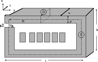 |
Table 1 lists the variable names along with typical values. Without typical
dimensions and material parameters, this design problem would continue to be an abstract
mathematical exercise.
Table 1:
Typical values for variables used.
| Geometry |
|
 m m |
Other |
|
|
| Yoke length |
 |
15 |
Relative permeability |
 |
3000 |
| Yoke width |
 |
20 |
Conductivity |
 |
5e6 |
| Stack height |
 |
10 |
Magneto-motive force |
 |
0.03 |
| Gap |
 |
0.1 |
Skin depth |
 |
|
| Pole thickness |
 |
3 |
Frequency |
 |
|
| Track width |
 |
0.25 |
Dissipation time |
 |
|
For starters, we assume that the material is isotropic and linear and separate the problem
into two components
- Static case ...when a constant high current is applied to the coils and the
writer erases the magnetic disk e.g. while formating a drive.
- Dynamic case ...when we rapidly the direction of current in the coils so as to
write a pattern of 1's and 0's on the media.
The dynamic case, which requires a self-consistent solution to both Ampere's law around loop C
and Faraday's law around loop D, is somewhat complicated. Hence it also becomes necessary
to understand under what circumstances one can use the more convenient static approximation.
Referring to the closed loop C in Fig. 2, we write down Ampere's law
(differential and integral forms respectively) as
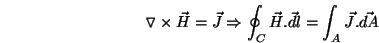 |
(1) |
The integral form is solved in terms of the fields at various points on the loop C. If we
assume that there is no leakage of magnetic flux i.e. all the field is concentrated within
the magnetic material. Following a flux line and expanding the above integrals yields
 |
(2) |
where, is the total magneto-motive force (MMF) obtained by adding all the current
traversing the area enclosed by C. (We currently ignore the change in width
of the pole pieces and close the contour before the nose).
A second relation between and  is obtained by solving the divergence equation
 across the gap. This merely yields a continuity
equation (see Sec 5.4.2, Ref 2) of the form
across the gap. This merely yields a continuity
equation (see Sec 5.4.2, Ref 2) of the form
 |
(3) |
Combining (2) and (3) yields the deep gap field
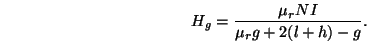 |
(4) |
Finally, the efficiency of the writer is defined to be
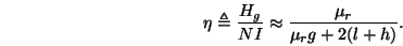 |
(5) |
We have thus illustrated the use of Ampere's law and an application of the divergence
theorem
 .
.
The reader is referred to Chap. 5 of Ref. 2 and the sub-sections below for a
theoretical basis of the following discussion.
Consider the rectangular cross-section of the top pole denoted by the closed
loop D in Fig. 2. Assuming a time variation of the form  , Faraday's law states that
 |
(6) |
Similarly, Ampere's law combined with
 becomes
 |
(7) |
where
 is the applied current density (in the coils),
 is the spatial distribution of the eddy current density and
 is the characteristic dissipation time for electric
charge within the conductor. The three terms for current density integral
arise from the external voltage applied to the writer coils, the electric field
due to a changing magnetic field (eddy current) and the magnetic field due
to the changing electric field (displacement current). For good
conductors,
is the characteristic dissipation time for electric
charge within the conductor. The three terms for current density integral
arise from the external voltage applied to the writer coils, the electric field
due to a changing magnetic field (eddy current) and the magnetic field due
to the changing electric field (displacement current). For good
conductors,
 and the last term is safely ignored.
Since the material used is a good conductor, we expect that all electric
charges reside on the surface. Furthermore, eddy currents generated by the time
varying magnetic field will flow in rectangular loops
on the outer surface. The problem is to solve (6) and (7)
simultaneously. We illustrate two possible approaches to the problem.
- Assume pole pieces that are very wide (
 ) and the fields decay
exponentially within the material. With a skin depth
) and the fields decay
exponentially within the material. With a skin depth  in the
material we have an approximate form for the spatial distribution of the
magnetic field in the pole piece,
in the
material we have an approximate form for the spatial distribution of the
magnetic field in the pole piece,
 |
(8) |
where
 . In the low frequency limit,
 ,
,  and is uniform through the
material. Substitute
and is uniform through the
material. Substitute  in (6) to estimate
  and then
integrate (7) around loop C. The resulting equation is
and then
integrate (7) around loop C. The resulting equation is
where  is the field at the center of the pole and we used the
continuity conditions on the tangential component of
is the field at the center of the pole and we used the
continuity conditions on the tangential component of  to evaluate the
integral of . From the assumed spatial distribution of , we also get
to evaluate the
integral of . From the assumed spatial distribution of , we also get
 Combining this with
![$H_g = \mu_r H\;\mathrm{and}\;\eta=\mathrm{Re}[H_g]/(NI)$](img52.png) we finally obtain the dynamic writer efficiency
we finally obtain the dynamic writer efficiency
![\begin{displaymath}
\eta (\omega) \approx \mathrm{Re}\left[\frac{\mu_r \mathrm{s...
...gamma
t/2)}{2(l+h)+g \mu_r \mathrm{sech}(\gamma t/2)}\right].
\end{displaymath}](img53.png) |
(11) |
It is instructive to note that we never quite used in our
calculation. However, the power loss due to the formation of
eddy currents depends on the spatial distribution of eddy currents which are
uniquely determined by and (7). Furthermore, we could have
derived  , under the approximation , from the static
expression (5) by defining
, under the approximation , from the static
expression (5) by defining
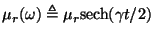 .
.
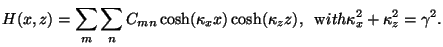
- Use separation of variables to find a series expansion for
 in a
rectangular cross-section and use the lowest order terms to solve
(1). Taking the origin at the center of the rectangle and from the
symmetry of the expected solution, we assume a solution to Helmholtz's equation
with the form
in a
rectangular cross-section and use the lowest order terms to solve
(1). Taking the origin at the center of the rectangle and from the
symmetry of the expected solution, we assume a solution to Helmholtz's equation
with the form
 |
|
|
(12) |
The coefficients  are to be determined by the boundary conditions
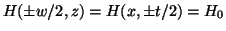 . Most text book
problems take advantage of the fact that the field or potential is zero on
one or more edges to determine the propagation constants. However this not
being the case here and with
. Most text book
problems take advantage of the fact that the field or potential is zero on
one or more edges to determine the propagation constants. However this not
being the case here and with  being complex, we do not have any obvious
choices for
being complex, we do not have any obvious
choices for  or
or  .
.
Both the time and spatial scales play an important role in problems with harmonic
excitations. Note that
- decreases as
 increases and it
gets harder to design writers as we operate at higher frequencies.
increases and it
gets harder to design writers as we operate at higher frequencies.
- decreases as increases since high resistivity materials restrict the
flow of eddy currents.
- increases with , though the increase is not quite as strong as in the
static case.
- The effective permeability
 decreases as the thickness
  of the
pole pieces increases.
of the
pole pieces increases.
Before we attack the problem of oscillating excitation currents in the writer coils, it is
imperative that we understand when the proposed dynamic solutions are valid. The
continuity equation for free charge is combined with Gauss' law to yield
 |
(13) |
where we assumed that the medium was homogeneous. Further assuming a linear medium, we find
that
 |
(14) |
Hence, we obtain a characteristic diffusion time
which
is the time it takes for charge to flow out to the surface of the conductor. For
our dynamic solution to be valid, one can adopt a rule of thumb that the write
current must switch directions over a time scale at least 100 times larger than
, such that
. This would allow the formation of eddy
current loops and permit an approximation of exponentially decaying
fields in the interior of the material, while ignoring the displacement
current.
For time harmonic (of the form ) excitations, combining the curl of the
differential equation in (1) with (6) and Ohm's law yields Helmholtz's
equation,
 |
(15) |
Fields propagating along  have solutions to the above equation of the
form
have solutions to the above equation of the
form  . The complex propagation constant has a real
component that relates to the exponential decay of fields within matter, while
the imaginary component represents the time harmonic solution.
For good conductors,
. The complex propagation constant has a real
component that relates to the exponential decay of fields within matter, while
the imaginary component represents the time harmonic solution.
For good conductors,
The skin depth
 is a measure of the distance it
takes for the electromagnetic field to decay to
is a measure of the distance it
takes for the electromagnetic field to decay to  of its original
value. The subscript is used explicitly to remind us that the skin depth depends
on the frequency of the electromagnetic excitations. Given a field
of its original
value. The subscript is used explicitly to remind us that the skin depth depends
on the frequency of the electromagnetic excitations. Given a field  at the
surface of the pole, we expect a solution that decays away from the surfaces of
the of the material and has a form
at the
surface of the pole, we expect a solution that decays away from the surfaces of
the of the material and has a form
![$H(x,t) = H_0 Re[e^{-\gamma y + j\omega t}] = H_0 e^{-x/\delta}\cos(x/\delta -
\omega t)$](img79.png) .
.
Next: Numerical Methods
Up: EC301: Electromagnetic Fields
Previous: A thematic approach
Anil Prabhakar
2002-09-25
![$\displaystyle NI-[2(l+h)-g]\int^{t/2}_0 J_e(x)dy,$](img46.png)