This module introduces a popular algorithm to implement constrained optimization, the so called projected gradient method (PGD). As the name suggests, this approach assumes that it is possible to compute gradients of the objective function. In case this is not possible or too expensive to do so, other approaches need to be considered, such as Nelder-Mead, coordinate search, or COBYLA (Constrained Optimization BY Linear Approximations).
Formulation of the PGD
The constrained problem we are trying to solve is:
and we start by recalling the simple gradient descent method, which follows these steps:
The PGD is very similar, with a simple projection step added after \(x_k\) update:
Here, we define the projection operator as:
i.e. find the point in \(\Omega\) closest to \(x_o\) (which may itself be in or out of \(\Omega\)). We note a couple of points in relation to PGD: * PGD is useful if \(P_{\Omega}()\) is easy to solve. * If \(\Omega\) is convex, then there exists a unique solution to the projection operation. Else, uniqueness is not guaranteed.
Graphical interpretation of projection
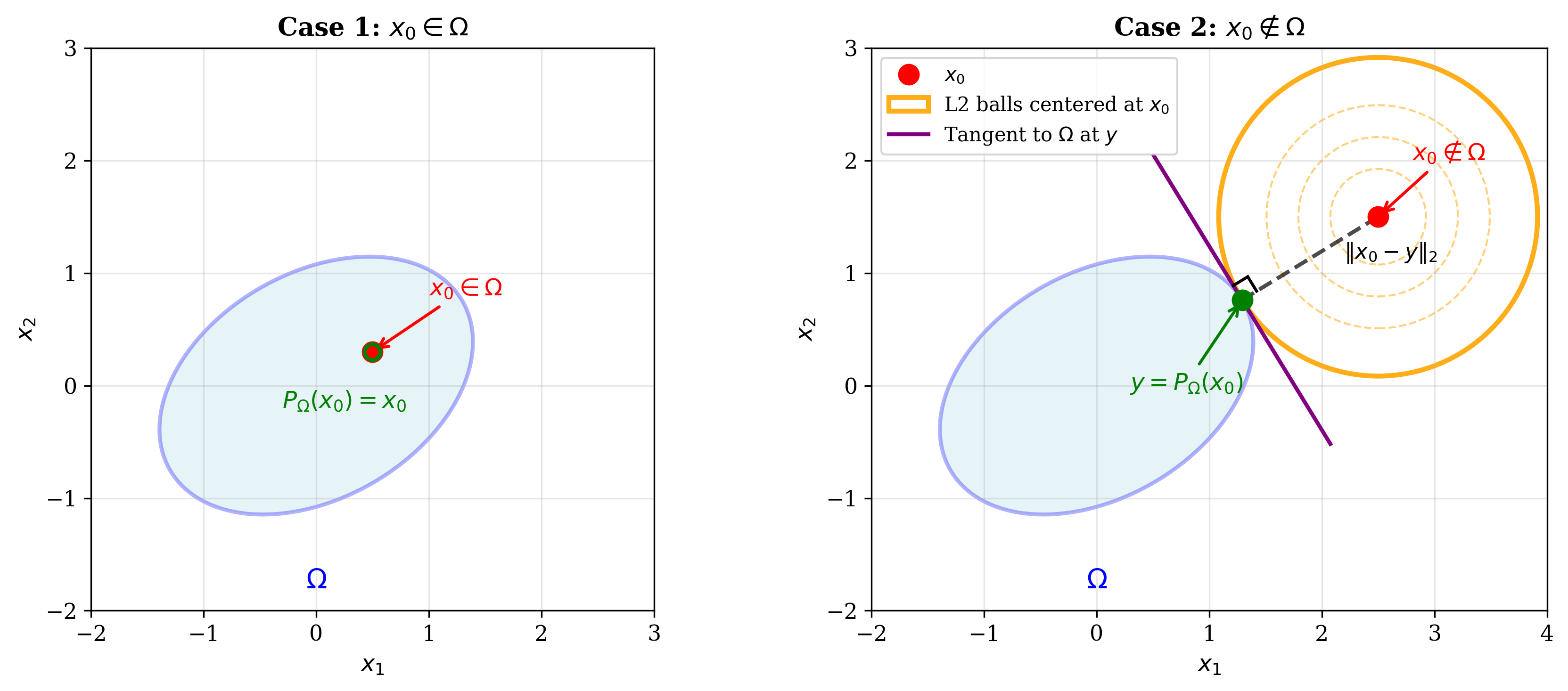
It is easy to see that when \( x_0 \in \Omega \), we get back the original point by applying \(P_{\Omega}()\).
However, when \( x_0 \notin \Omega \), we can conceive of L2 balls, centred at \(x_0\), and of increasing radius till the time they touch \(\Omega\) at some point \(y\). It can be shown that the line connecting \( x_0\) and \(y\) is perpendicular to the tangent to \(\Omega\) at \(y\).
Convergence of the PGD
While the suggested modification of the gradient method is intuitive, a very important question is if the method is actually guaranteed to converge. Indeed, the method does converge with a rate of convergence similar to that of gradient descent.
Proof
We will prove it for the simple case of a fixed step size, \(\alpha\).
For a convex function \(f\), we have for \(t \in [0,1\)]:
Set \(x = x^*\) (the optimal solution) and \(z = x_k\) (the current iterate). Then:
The PGD update is:
Therefore:
Using the simple result that \(\|p - q\|^2 = \|p\|^2 + \|q\|^2 - 2p^Tq\) for \(p, q \in \mathbb{R}^n\):
Let \(p = x_k - x^*\) and \(q = x_k - y_k\):
Since \(\|y_k - x^*\|^2 \geq \|x_{k+1} - x^*\|^2\) (by the projection property):
Telescoping this series from \(k=0\) to \(k=K-1\):
The second term is non-negative, so we can drop it:
Dividing both sides by \(K\):
By Jensen’s inequality for convex functions:
Therefore:
This shows that on average, we converge to the optimal solution. The rate of convergence is similar to that of gradient descent, namely \(O(1/K)\).
Example: projection on the unit ball
If \(\Omega = \|x\|^2_2 \leq 1\) is the unit ball, then what is \(P_{\Omega}(x_o)\)?
Of course, in case \(x_o\in\Omega\) then \(P_{\Omega}(x_o)= x_o\). For the next case, using the geometric intuition provided earlier, we can see that the projected point will be on the surface of the unit ball on the line from the origin to \(x_o\). Mathematically: \(P_{\Omega}(x_o) = x_o / \|x_o\|_2\).
So, we can combine both cases and write the projection operation as:
Extra: prove the above by using the Lagrangian and KKT conditions for practice.
Some common projection operations
Let \(\Omega = \{x : \|x\|_2 \leq 1\}\), which is a convex optimization problem. Then the projection operation is:
which can be compactly written as:
Homework: Prove this using the Lagrangian and KKT conditions.
Motivation: When you solve this problem you will realize that we need to take gradients of the Lagrangian. When \(\Omega\) is the L1 ball, we will have problems when the gradient is not defined at certain points. This motivates the next topic of subgradients which can be defined when the gradient can’t be defined.
Subgradients
We will restrict our discussion to convex functions.
Definition and properties
For a differentiable convex function \(f\):
This is the first-order characterization of convexity - the function lies above its tangent plane at any point. In fact, \(f(x) + \nabla f(x)^T(y - x)\) is the supporting hyperplane for \(f\) at \(x\).
A subgradient of a convex function \(f\) at \(x\) is a vector \(g\) such that:
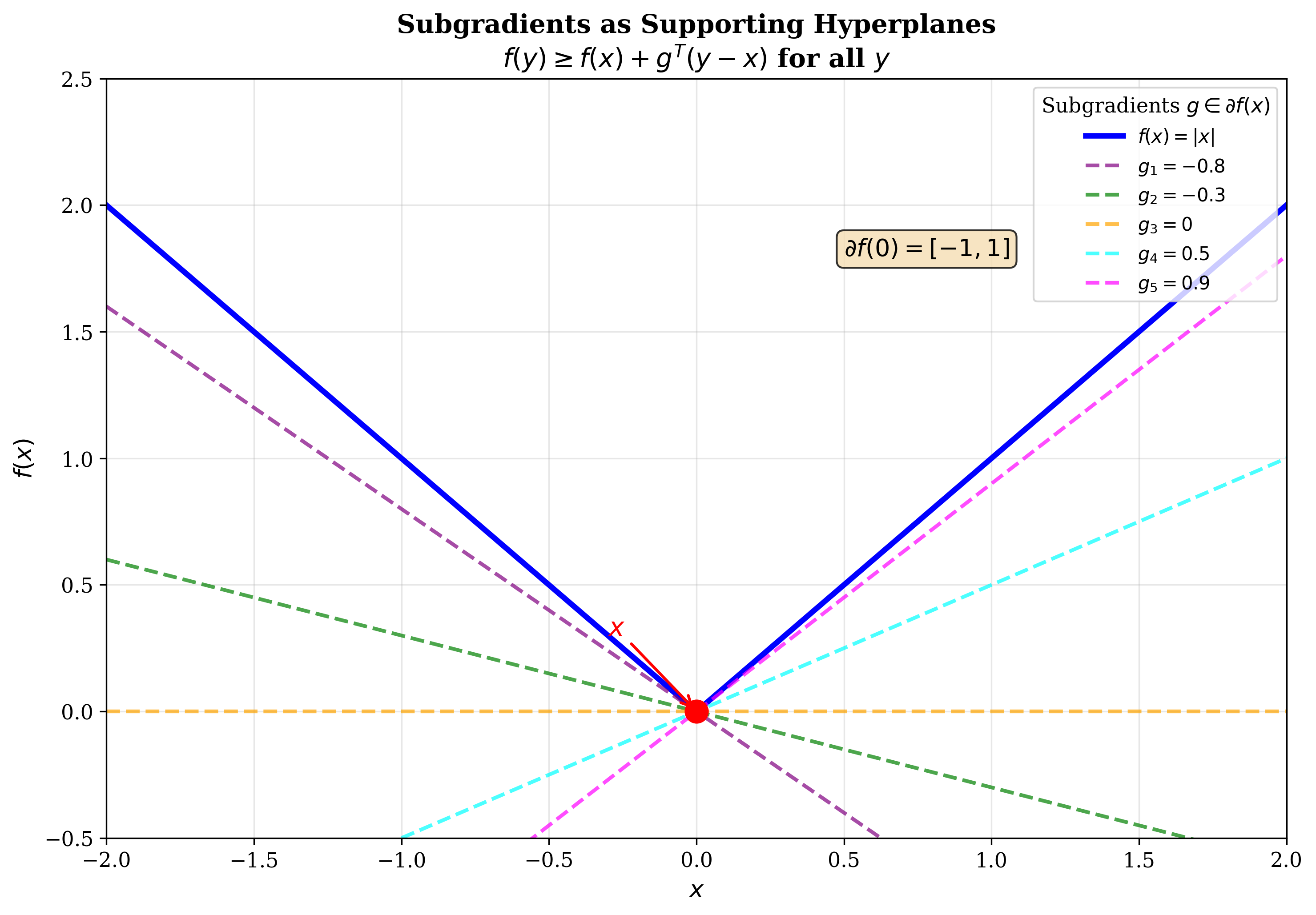
In the figure above, both \(g_1\) and \(g_2\) are subgradients at \(x\). They define supporting hyperplanes at \(x\), i.e., they never cut through the function’s graph.
The subdifferential is the set of all subgradients at point \(x\):
The subdifferential \(\partial f(x)\) is a closed convex set.
Examples
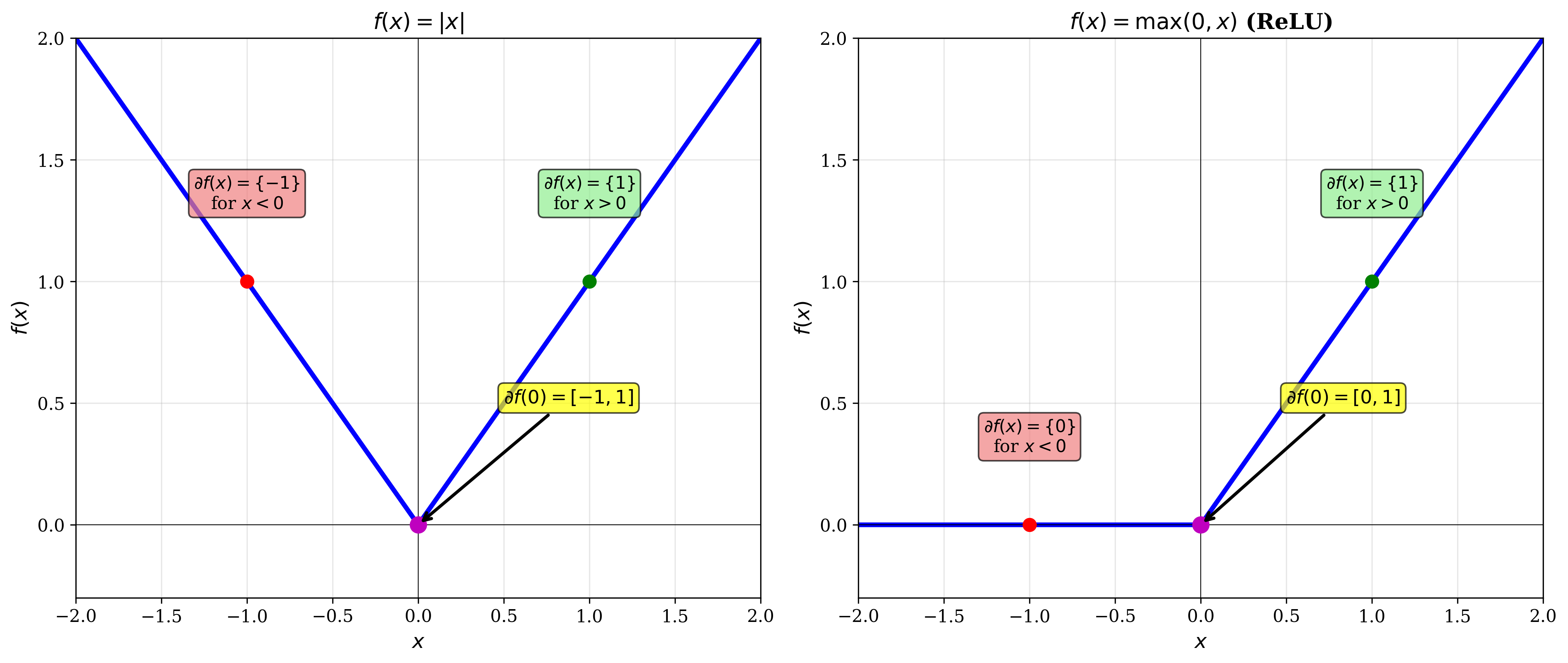
Example 1: \(f(x) = |x|\)
which can be compactly written as:
Example 2: \(f(x) = \text{max}(x, 0)\)
Use of subgradients
Subgradients provide a way of restating optimality conditions. For any function \(f\):
where the first equality states the usual understanding of \(x^*\) being an optimal point and the second part is the restatement of optimality.
Why is this true? If \(g=0\), then being a subgradient implies that \(f(y) \geq f(x^*) + g^T(y - x^*) \geq f(x^*)\), i.e. \(x^*\) is optimal.
This generalizes the familiar optimality condition \(\nabla f(x^*) = 0\) to non-differentiable functions.
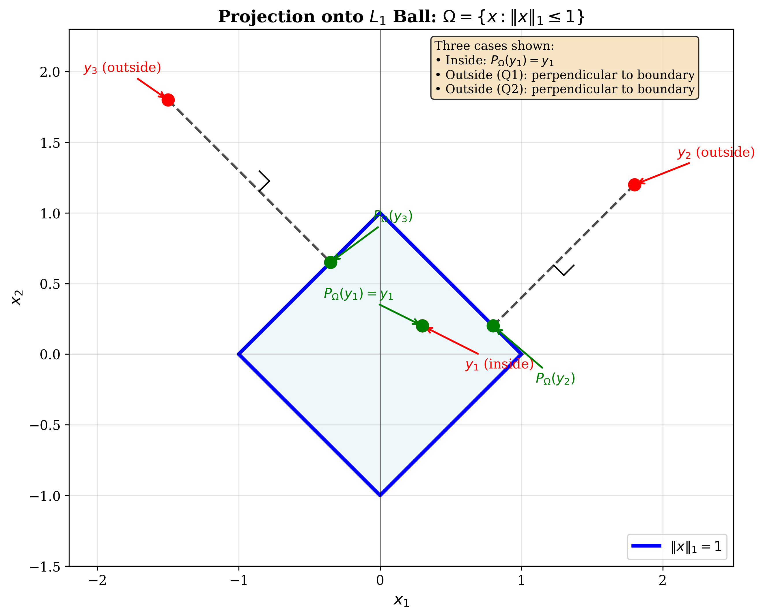
Projection onto the L1 ball
Consider the problem of projecting onto the L1 ball: \(\Omega = \{x : \|x\|_1 \leq 1\}\).
By definition, the projection problem is:
We can rewrite this in the language of constrained optimization like so:
where \(\lambda \geq 0\) is the Lagrange multiplier.
The Lagrangian is:
Taking the derivative with respect to \(x\):
Now, \(|x_i|\) is not differentiable when \(x_i = 0\), so we use subgradients:
where \(g_i \in \partial |x_i|\).
From the KKT conditions:
Case 1: \(\lambda = 0\) (\(x\) is inside or on the boundary)
This corresponds to the case where \(\|y\|_1 \leq 1\), so \(P_{\Omega}(y) = y\).
Case 2: \(\lambda > 0\) (\(x\) is on the boundary, \(\|x\|_1 = 1\))
From \(x_i - y_i + \lambda g_i = 0\):
-
If \(x_i > 0\): \(g_i = 1\), so \(x_i = y_i - \lambda\)
-
If \(x_i < 0\): \(g_i = -1\), so \(x_i = y_i + \lambda\)
-
If \(x_i = 0\): \(g_i \in [-1, 1\)], so \(y_i \in [-\lambda, \lambda\)]
We are free to choose any value of the subgradient from the subdifferential. If we set \(g_i = \text{sgn}(y_i)\), we get:
This is the soft-thresholding operator:
where \((t)_+ = \max(0, t)\).
Compactly:
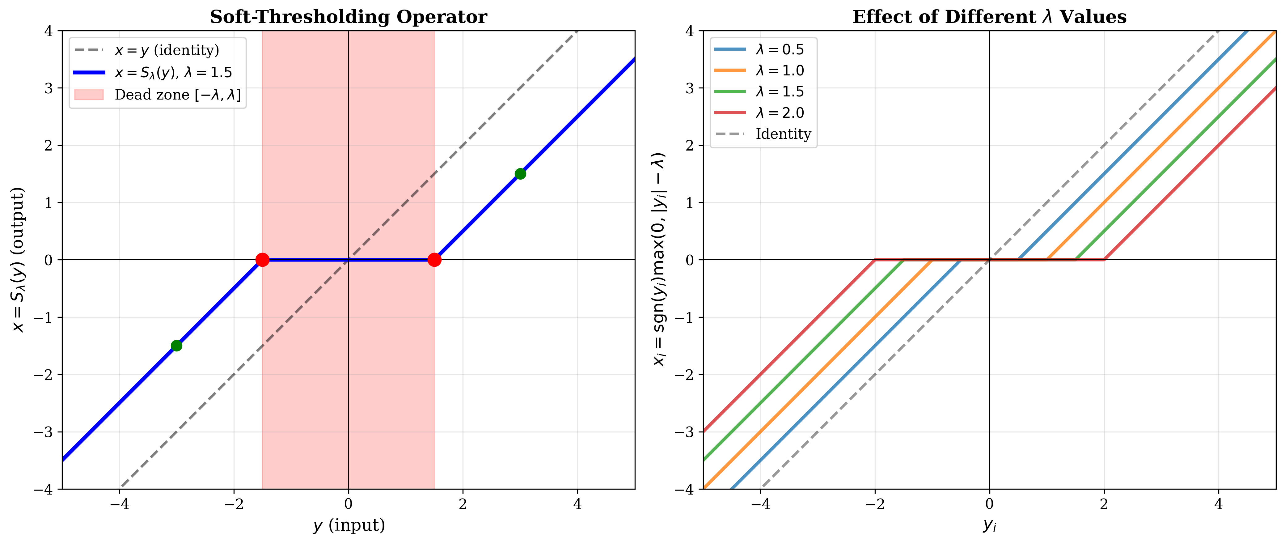
The soft-thresholding operator shrinks values toward zero by \(\lambda\) and sets small values exactly to zero (the "dead zone").
Finding \(\lambda\): We still need to determine \(\lambda\). From the KKT complementarity condition:
When \(\lambda > 0\):
This can be solved for \(\lambda\). Then finally, once we get \(\lambda\), we can get \(x\) as:
Example: Projection onto L1 ball
Example 1: Let \(y = (3, 2, 1)^T\) and we want \(P_{\Omega}(y)\) where \(\Omega = \{x : \|x\|_1 \leq 1\}\).
First, find \(\lambda\) from:
Try different values: - \(\lambda = 2.7\): \(\|x\|_1 = |3-2.7| + |2-2.7| + |1-2.7|_+ = 0.3 + 0.7 + 0 = 1.0\) ✓
Then:
Wait, let me recalculate: \(x = (0.3, 0, 0)^T\) gives \(\|x\|_1 = 0.3\), which doesn’t equal 1.
After projection: \(x_1 = 0.3, x_2 = 0, x_3 = 0.7\) (based on the handwritten notes).
Example 2: Let \(y = (13, 7, 9)^T\).
Finding \(\lambda\):
For \(\lambda\) in the range \([7, 9\)]:
But \(\lambda = 14 \notin [7, 9\)], so this doesn’t work.
The best possible choice is to go below 7. Let \(\lambda = 3.0\):
For large problems, this can be solved by sorting (see Condat’s solution, 2016).
Note: After the projection, we get: