In this module, we will explore the area of Constrained optimization (CO), largely based on Ch 12 of NW. Engineering abounds in CO problems — from maximizing the throughput of production given constraints on labour timings and electricity charges, to minimizing energy consumption of a device while maintaining a certain quality of service, to quote just a few examples.
Terminology
Feasible set
In the world of unconstrained optimization, a problem would simply be written as \( \underset{x}{\text{min}} f(x)\). Once we move into the world where constraints are placed on the optimization variable, \(x\), that notation changes to \( \underset{x\in\Omega}{\text{min}} f(x)\), where \(\Omega\) is called the feasible set, i.e. the set of `legal' \(x\) values that obey the constraints of the problem.
This is best illustrated via an example. Consider two constraints given as:
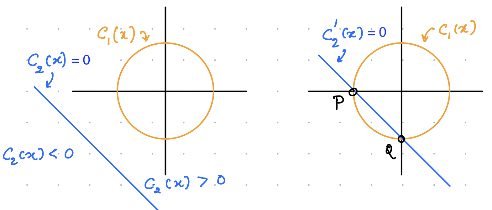
As seen in the figure on the left, the first constraint forces \(x\) to lie on the circle \(c_1\), whereas the second insists that \(x\) be in the top-right half-plane as defined by \(c_2\). Thus the feasible set, in this case, is just the set of points on \(c_1\). On the other hand, if we replace \(c_2\) by a new constraint of the form \(c_2'(x) = x_1 + x_2 +\sqrt{2} \ge 0\), then the feasible set changes to the part of the circle given by \(-\pi/2 \le \theta \le \pi\), as seen in the figure on the right.
In general, the constraints are expressed in the following form:
where the sets \(\mathcal{E},\mathcal{I}\) denote the sets of equality and inequality constraints, respectively.
Active set
Considering an inequality constraint defining the problem, a constraint is said to be `active' at a point \(x\) in \(\Omega\) if \(c_i(x) = 0\) at that point, else it is termed as inactive.
The active set at a point \(x\) in \(\Omega\), is defined as the union of equality and active inequalities, i.e. \(A(x) = \mathcal{E} \cup \{ i\in \mathcal{I} | c_i(x) = 0\}\). For example, in the above figure(left), \(A(x) = \{1\}\) at all points in the feasible set, whereas on the right, \(A(x) = \{1,2\}\) at points \(P,Q\), and \(A(x) = \{1\}\) everywhere else in the feasible set. Note the "1" and "2" refer to the subscripts on the constraints, \(c_1,c_2\), respectively.
Examples to build intuition
Single equality constraint
We now introduce the idea of constrained optimization by starting with the simple case of a single equality constraint. Say that the objective function we wish to minimize is \(f(x) = x_1 + x_2\) subject to \(c_1(x) = x_1^2 + x_2^2 -2 =0\).
Geometric intuition
It is worthwhile to plot the function and constraints because doing so gives us geometric intuition into some general principles as we will see. As is evident from the figure the solution to this problem is given by the point \(A\). Let’s see how we can arrive at this via a formal method.
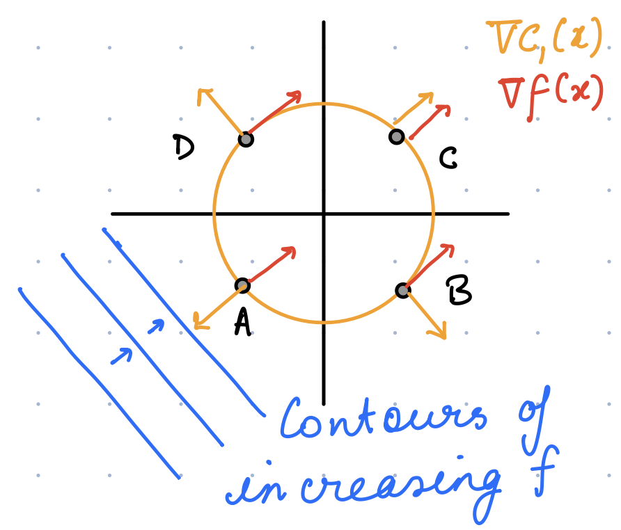
We start by considering the gradients of the function and constraints, i.e. \(\nabla f(x) = [1,\, 1]^T\) and \(\nabla c_1(x) = 2 [ x_1,\, x_2]^T\), which are also plotted in the figure above. Evidently, at the solution point \(A\), both \(\nabla f\) and \(\nabla c_1\) are parallel to each other, so we conjecture that at the solution, we could write \(\nabla f(x^*) = \lambda_1 \nabla c_1(x^*)\), where \(\lambda_1\) is some scalar. However, we can immediately see that this condition also seems to hold at the point \(C\).
Calculus formalism
Let us now make this intuition more formal. Let’s say that we are in the process of optimizing our function and find ourselves at a feasible point \(x\in\Omega\). We would like to move to another feasible point \(x+s\) which improves the objective function. Explicitly, these are the qualities of the new point:
-
The point stays feasible, i.e. \(c_1(x+s) = 0\). By Taylor’s theorem to first order, this implies \(c_1(x+s) = c_1(x) + \nabla c_1(x)^Ts\), which in turn implies \(\nabla c_1(x)^Ts=0\).
-
The point improves the objective function value, i.e. \(f(x+s) < f(x)\). Again by Taylor’s theorem to first order, we write \(f(x+s) = f(x) + \nabla f(x)^T s\), which in turn implies \(\nabla f(x)^Ts < 0\).
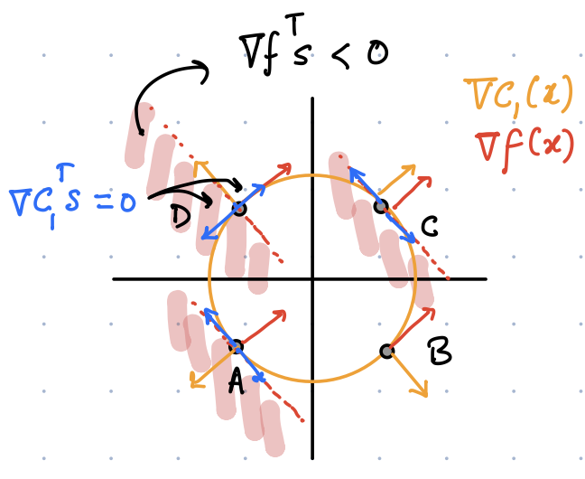
Thus as long as an \(s\) can be found, I can keep reducing the objective function value, as seen in the point \(D\) in the figure above. The natural question to ask is: When will it be impossible to move further? Let us see figure above. Evidently, at both points \(A\) and \(C\), it is not possible to simultaneously satisfy both criteria. Thus, we state that the possible signature of a local minima is:
We now introduce a "Lagrangian" function, defined like so: \(\mathcal{L}(x,\lambda_1) = f(x) - \lambda_1 c_1(x)\), where \(\lambda_1\) is referred to as the Lagrange multiplier for \(c_1\). When we evaluate the gradient of the Lagrangian w.r.t. the variable \(x\), i.e. \(\nabla_x \mathcal{L}(x,\lambda_1) = \nabla f(x) - \lambda_1 \nabla c_1(x)\), we see that the expression that we had derived earlier (for a minima) can also be arrived at the following recipe, referred to as a necessary condition for a stationary point:
Single inequality constraint
In the next example, we take up the case of an optimization problem with a single inequality constraint. Let us consider the same objective function \( f(x) = x_1 + x_2\) subject to the constraint \(c_2(x) = 2-x_1^2 -x_2^2 \ge 0\).
Let us say that we are at a feasible point \(x\), and wish to go to \(x+s\) to improve our objective function further while staying feasible. We thus have:
(1) \(c_2(x) \ge 0\). From Taylor’s theorem we get \(c_2(x+s) = c_2(x) + \nabla c_2(x)^Ts \ge 0\), and
(2) the improvement criteria which leads to \(\nabla f(x)^Ts < 0\).
To make the analysis simpler, let us split the possibilities into two:
-
Case 1: the constraint is inactive, i.e. \(c_2(x) > 0\), and
-
Case 2: the constraint is active, i.e. \(c_2(x) = 0\).
In case 1, we see that \(c_2(x) + \nabla c_2(x)^Ts \ge 0\) is the requirement, and since \(c_2(x)>0\), any sufficiently small \(s\) will still satisfy the above condition. For e.g. setting \(s = -\alpha \nabla f\) with a judicious choice of \(\alpha\) is good enough as it also satisfies the improvement criteria, \(\nabla f(x)^Ts < 0\).
In case 2, we see that \(c_2(x) = 0\), and so the requirement becomes \(\nabla c_2(x)^T s \ge 0\), in addition to the existing requirement of \(\nabla f(x)^Ts < 0\).
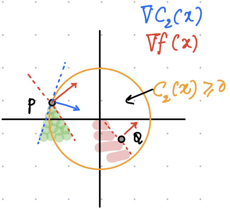
Both cases can be seen graphically above; in case 1 (point \(Q\)), any \(s\) in the open half-space (\(\nabla f(x)^Ts < 0\)) is good enough, while in case 2 (point \(P\)), a possible solution can be found in the intersection of the closed half-space (\(\nabla c_2(x)^T s \ge 0\)) and the open half-space (\(\nabla f(x)^Ts < 0\)).
Stopping criteria
In other words, when is it not possible to find any \(s\) that satisfies the above criteria? Again, let’s analyze both cases separately. No feasible direction \(s\) will result:
-
In case 1 (where \(c_2(x) > 0\)), if \(\nabla f(x) = 0\). In the language of the Lagrange function, this means \(\nabla_x \mathcal{L}(x,\lambda_2) = \nabla f(x) - \lambda_2 \nabla c_2(x)=0\) and \(\lambda_2 = 0\).
-
In case 2 (where \(c_2(x) = 0\)), the two half-spaces don’t have any points in their intersection. Graphically, we see this happening at point \(A\) when the two gradients, \(\nabla f\) and \(\nabla c_2\) are parallel (not even anti-parallel), i.e. \(\nabla f(x^*) = \lambda_2 c_2(x^*)\) for \(\lambda_2 \ge 0\). In the language of the Lagrange function, this means \(\nabla_x \mathcal{L}(x,\lambda_2) = \nabla f(x) - \lambda_2 \nabla c_2(x)=0\) and \(\lambda_2 \ge 0\).
Both these cases can be neatly combined as follows: For optimising a function with a single inequality constraint, we have the following necessary conditions for a local minima:
Two inequality constraints
An example.
Algebra v/s geometry
While we have not yet discussed any algorithms for constrained optimization, it is natural to think about legitimate directions of progress in the course of optimization. We have referred to these directions as feasible directions and they ensure that we always stay in the feasible set as defined by the constraints of the problem. Note the difference with unconstrained optimization, where our only consideration was to achieve a decrease in the objective function value. In the case of constrained optimization, we need to maintain feasibility in addition.
Linearised feasible directions
In the preceding discussion, we used the first order Taylor’s theorem to sketch out the possible feasible directions. These are formally called as the set of linearised feasible directions, defined like so:
\( \mathcal{F}(x) = \left\{ d \, \Bigg| \begin{aligned} d^T\nabla c_i(x) = 0 & \forall i \in \mathcal{E} \\ d^T \nabla c_i(x) \ge 0 & \forall i \in \mathcal{A} \cap \mathcal{I} \end{aligned} \right. \)
Note that the second line consists only of those inequality constraints that are active. As we saw previously, for the case of inactive inequality constraints, any small vector is a feasible direction and hence is not included in the above set.
Let us now revisit a previous example of equality constraint, i.e. \(f(x) = x_1 + x_2\) and \(c_1(x) = x_1^2 + x_2^2 -2 = 0\). Here, simply by geometry we know the solution to be \((-\sqrt{2}, -\sqrt{2})\).
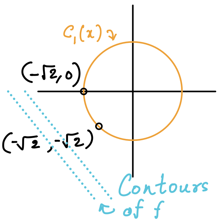
Now, consider the point \((-\sqrt{2},0)\) (see figure above). By definition, \( \mathcal{F}(x) = \{ d | d^T\nabla c_1(x) = 0\} \), which translates to:
\( \begin{bmatrix} d_1 & d_2\end{bmatrix} \begin{bmatrix} 2x_1 \\ 2x_2\end{bmatrix} = -2\sqrt{2} d_1 = 0, \quad \implies \mathcal{F}(x) = \left\{ \begin{bmatrix} 0 \\ d_2 \end{bmatrix} | \, d_2 \in\mathbb{R} \right\} \).
Thus, at \((-\sqrt{2},0)\) the set of linear feasible directions correspond to any vector in the \(\pm x_2\) direction. This aligns with our intuition as a move in the \(-x_2\) direction will take us towards the solution of the problem.
A problem with algebra
Instead of the constraint being specified as \(c_1(x) = x_1^2 + x_2^2 -2 = 0\), let’s see what happens if it was specified as \(c_1(x) = (x_1^2 + x_2^2 -2)^2 = 0\). Geometrically, we can see that the feasible set is unchanged — it is still the set of all points on the circle. However, due to the algebraic change in the constraint specification, do the linearised feasible directions change? In this case, we have:
\( \mathcal{F}(x) = \{ d | d^T\nabla c_1(x) = \begin{bmatrix}d_1 & d_2 \end{bmatrix} \begin{bmatrix} 4(x_1^2+x_2^2-2)x_1 \\ 4(x_1^2+x_2^2-2)x_2 \end{bmatrix} = 0 \}\), which is satisfied by any \(d_1,d_2 \in \mathbb{R}\) at \((-\sqrt{2},0)\). Thus, \( \mathcal{F}(x) = \mathbb{R}^2\), i.e. any direction is feasible as per this definition even though the geometry is unchanged.
Thus a change in the algebraic specification has led to an erroneous set of feasible directions. In order to "tighten" this gap between algebra and geometry, we need something extra. This "extra" bit is called "constraint qualification" — these are assumptions that ensure similarity of the constraint set \(\Omega\) and its linearised approximation at \(x\). Before we get to these, we need to define a few geometric entities.
Geometric tools
Just as in the case of algebraic specifications we came up with a formal definition of linearised feasible directions, similarly we need a formal tool in the case of geometric specifications. This tool is called the tangent cone. In order to get to it, we need a few definitions:
-
Feasible sequence — Given a point \(x\) in the feasible set \(\Omega\), \(\{z_k\}\) is a feasible sequence if \(z_k \in \Omega\) for large \(k\), and \( \lim_{k\to\infty} z_k \to x\).
-
Local minimiser — This is a point \(x\in\Omega\) at which all feasible sequences have the property that \(f(z_k) \geq f(x)\) for large \(k\). For example, consider \( f(x) = x_1 + x_2\) and \(c_1(x) = x_1^2 + x_2^2 -2 = 0\) and two sequences \(S_1, S_2\) which approach the point \(A = (-\sqrt{2},0)\) for large \(k\), also shown graphically in the figure below. \(S_1\) is defined as \(z_k = \{(-\sqrt{2-\frac{1}{k^2}}, \, \frac{1}{k})\}\), while \(S_2\) is defined as \(w_k = \{(-\sqrt{2-\frac{1}{k^2}}, \, -\frac{1}{k})\}\). Clearly, for large values of \(k\), we have both \( \{z_k,w_k\} \to A\) for \(k\geq 1\). However, it is also true that \(f(z_k) > f(A)\) for \(S_1\), while \(f(w_k) < f(A)\) for \(S_2\). Thus, \(A\) is not a local minimiser for this problem.
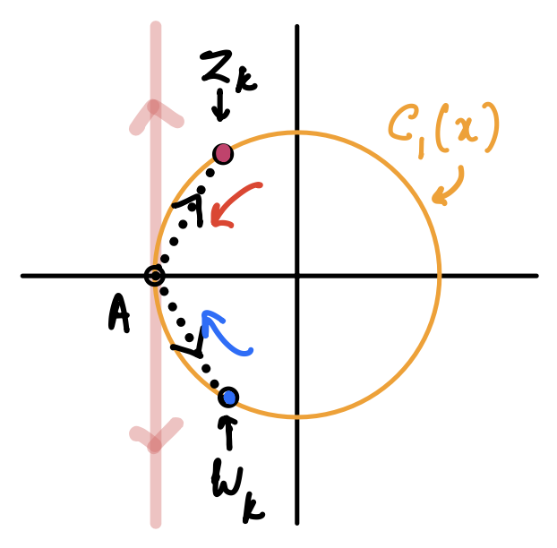 Figure 6. Feasible sequences and tangent cones
 -
Tangent — A tangent is a limiting direction of a feasible sequence. In addition to \(\{z_k\}\) we also define a sequence of positive scalars, \(\{t_k\}\) with the property that \( \lim_{k\to \infty} t_k \to 0\). Among many candidates, \(t_k = \|z_k - x\|_2 \) is suitable since it satisfies the just mentioned property. Note that there can be several possible ways of defining \(t_k\) that is left to us. Then, a tangent, \(d\), is defined as: \( d= \lim_{k\to\infty} \frac{z_k - x}{t_k}\).
-
The tangent cone is defined as the set of all tangents to \(\Omega\) at a feasible point \(x\), denoted as \(T_{\Omega}(x)\). As an aid to visualisation, one imagines standing at \(x\) and watching a feasible sequence \(\{z_k\}\) approach you. The limiting direction (the approaching vector, \(z_k-x\), divided by the scalar, \(t_k\)) gives us a tangent (see the dashed arrows in the figure above). Now we collect all possible tangents that arise from the set of all feasible sequences, and we have our tangent cone. In our example above, if we chose the feasible sequence as \(t_k = \|z_k-x\|_2\), for either of the sequences \(S_1,S_2\), we get the tangents \( [0,\pm 1]^T\). However, there is considerable freedom in choosing \(t_k\), for e.g. \(t_k = 1.22 \|z_k-x\|\) works just as well. Thus we find that if we collect all possible tangents, the resulting tangent cone we get is \( T_{\Omega}(A) = \begin{bmatrix} 0 \\ d_2 \end{bmatrix}, d_2 \in \mathbb{R}\).
Why is the tangent cone a cone?
-
A cone is defined as a set \(M\) which has the property that for \(\forall x \in M\), we also have \(\alpha x \in M, \forall \alpha>0\).
-
The set defined as \( \{(x_1,x_2) | x_1, x_2 > 0 \}\) is an example of a convex cone, where as the set defined as \( \{(x_1,x_2) | x_1\geq 0 \text{ OR } x_2 \geq 0 \}\) is an example of a non-convex cone (sketch and confirm)].
-
Why do we call the tangent cone a cone? We just have to check if \(d \in T_{\Omega}(x)\), then is \(\alpha d \in T_{\Omega}(x)\)? This is easy enough to prove due to the freedom in choosing the feasible sequence \(t_k\). For e.g. if we choose \(t_k' = t_k/\alpha\), then it follows that \(\alpha d\) is also a tangent, and hence it is in the tangent cone.
Constraint qualifications
We define linear independence constraint qualification (LICQ) in the following way: Given a feasible point \(x\) and the active constraint set \(\mathcal{A}(x)\), we say that LICQ holds if the set of active constraint gradients, \(\{\nabla c_i(x) | i \in \mathcal{A}(x)\}\) is linearly independent.
Having defined the geometric points above, we are in a position to bridge algebra and geometry due to the following two true statements:
-
The tangent cone, \(T_{\Omega}(x)\), is a subset of the set of linearised feasible directions, \(\mathcal{F}(x)\).
-
More importantly, if LICQ holds, then \(T_{\Omega}(x) = \mathcal{F}(x)\) (see proof in NW, lemma 12.2).
As validation, consider the example above once again, where \( T_{\Omega}(A) = \begin{bmatrix} 0 & d_2 \end{bmatrix}^T, d_2 \in \mathbb{R}\). We can see that when the constraint is defined as \(c_1^2(x) + c_2^2(x)-2=0\), we had \(\mathcal{F}(x) =\begin{bmatrix} 0 & d_2 \end{bmatrix}^T, d_2 \in \mathbb{R}\). In this case, \(\nabla c = \begin{bmatrix} -2\sqrt{2} & 0 \end{bmatrix}^T\). Since this vector is non-zero, it is legitimate to consider it as a set of linearly independent vectors. Whereas, when we defined the constraint like so: \((c_1^2(x) + c_2^2(x)-2)^2=0\), we get \(\nabla c = \begin{bmatrix} 0 & 0 \end{bmatrix}^T\), which is clearly not linearly independent.
Thus, LICQ is helping us identify when to not be misled by a certain algebraic specification. In most cases it is easier to work with algebraic specification (all I have to do is compute gradients), rather than construct all possible feasible sequences to compute a tangent cone, thus underlining the importance of LICQ.
First order necessary conditions
Having studied several examples to build intuition, and armed with constraint qualification tools, we can now formalise the theorem for first order necessary conditions (FONC) of constrained optimization, also known popularly as the Karush Kuhn Tucker (KKT) conditions (after the co-discoverers).
Theorem statement
As before, the Lagrangian is defined as: \( \mathcal{L}(x,\lambda) = f(x) - \sum_i \lambda_i c_i(x), \quad i \in \mathcal{E} \cup \mathcal {I}\). The theorem below give us a first order test to check for the optimality of a candidate point \(x^*\).
-
\(x^*\) is a local solution of the problem,
-
the objective function \(f\) and the constraints \(c_i\)'s are continuously differentiable,
-
LICQ holds at \(x^*\),
-
\(\nabla_x \mathcal{L}(x^*,\lambda^*) = 0\),
-
\(c_i(x^*) = 0, \, \forall i \in \mathcal{E}\),
-
\(c_i(x) \geq 0, \, \forall i \in \mathcal{I}\),
-
\(\lambda_i \geq 0, \, \forall i \in \mathcal{I}\),
-
\(\lambda_i \, c_i = 0, \, \forall i \in \mathcal{E} \cup \mathcal {I}\), the complementarity conditions.
There can be many points where the above hold, however, with LICQ, the optimal \(\lambda^*\) is unique.
Instead of giving a general proof, we will give a proof sketch by working with an example.
Proof sketch
The problem is to minimise \(f(x) = x_1 + x_2\) subject to \(c_1(x) = 2 - x_1^2 - x_2^2 \geq 0\) and \(c_2(x) = x_2 \geq 0\). We will list out the implications of the FONC that apply to a candidate point \(x\) in order for it to be a local minima.
Obviously, the point under consideration must be feasible, so \(c_1(x) \geq 0\) and \(c_2(x) \geq 0\) must hold. We can further divide the possibilities as follows, and list out the FONC as per the theorem:
-
If \(c_1(x) =0\) and \(c_2(x) = 0\), then \(\nabla f(x) - \lambda_1 \nabla c_1(x) - \lambda_2 \nabla c_2(x) = 0\) and \(\lambda_1 \geq 0\), \(\lambda_2 \geq 0\).
-
If \(c_1(x) > 0\) and \(c_2(x) = 0\), then \(\nabla f(x) - \lambda_2 \nabla c_2(x) = 0\) and \(\lambda_1 = 0\), \(\lambda_2 \geq 0\).
-
If \(c_1(x) = 0\) and \(c_2(x) > 0\), then \(\nabla f(x) - \lambda_1 \nabla c_1(x) = 0\) and \(\lambda_1 \geq 0\), \(\lambda_2 = 0\).
-
If \(c_1(x) > 0\) and \(c_2(x) > 0\), then \(\nabla f(x) = 0\) and \(\lambda_1 = 0\), \(\lambda_2 = 0\).
We will now sketch the proof for case (1) above, step-by-step:
-
We need to show that \(\nabla f(x) = \lambda_1 \nabla c_1(x) + \lambda_2 \nabla c_2(x)\) for \(\lambda_1 \geq 0,\, \lambda_2 \geq 0\). In fact, we can easily recognise the geometric region that is being indicated here, namely a cone. That is, we need to show that \(\nabla f(x)\) must live in a cone defined by two vectors, \(\nabla c_1(x),\, \nabla c_2(x)\) (see figure below). Let’s formally define this cone as:
\( A : \{ u\in\mathbb{R}^2: u = \lambda_1 \nabla c_1(x) + \lambda_2 \nabla c_2(x), \, \lambda_1, \lambda_2 \geq 0 \}\)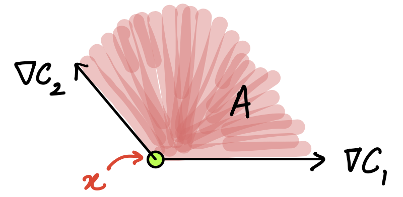 Figure 7. Cone formed by constraint gradients
What are the linearised feasible directions in this case? They are given by the intersection of \(\nabla c_1^T d\geq 0\) and \(\nabla c_2^T d\geq 0\), i.e. two half spaces, which are sketched below in the figure:
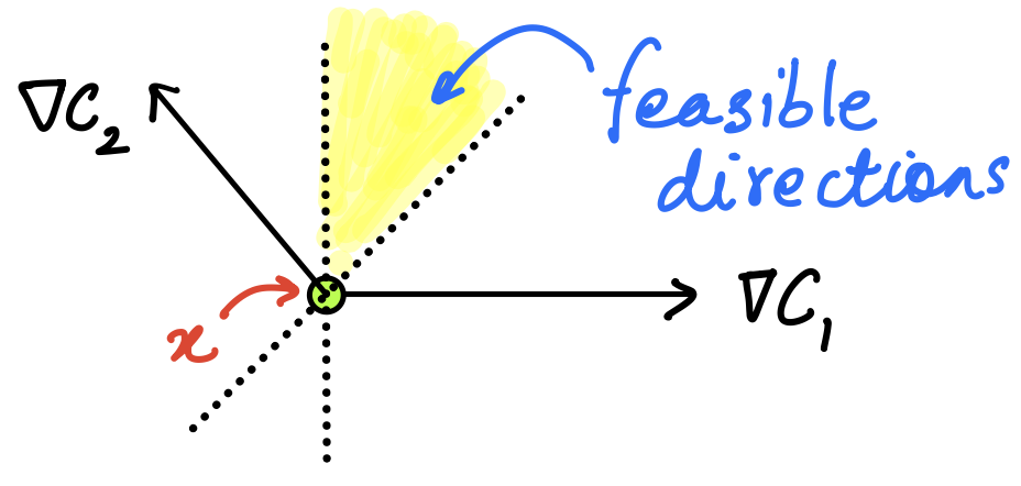 Figure 8. Linearised feasible directions forming a cone
 -
We will prove this by contradiction, i.e. assume that \(\nabla f \notin A\).
-
Since \(\nabla f\) is outside \(A\), we find a point \(s\) from \(A\) that is nearest to \(\nabla f\), i.e. \(s = \text{argmin}_{w\in A} \|w - \nabla f\|\) and shown in the figure below. Having found this point, we will claim that the direction given by \(s-\nabla f\) is both, feasible, AND a descent direction. If this is found to be true, then it would imply that \(x\) can be improved by moving along this direction, contradicting the starting proposition of \(x\) being a local minima.
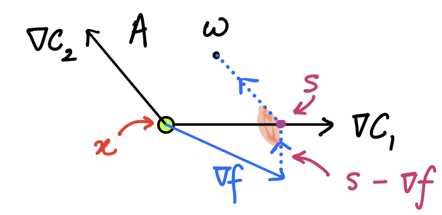 Figure 9. Investigation of \(s-\nabla f\)
 -
What are the arguments for the claim regarding \(s - \nabla f\)?
-
Since the point \(s\) has been obtained as a projection of \(\nabla f\) on \(A\), it follows that \(\|s\| \leq \| \nabla f\|\). And so, we can see that \( s^T\nabla f < (\nabla f)^T \nabla f\). This leads to \((s-\nabla f)^T \nabla f < 0\), which implies that \(s-\nabla f\) is a descent direction.
-
For the claim of feasibility, we start by asserting (but not proving), a property of convex sets that’s quite intuitive. Consider any point \(w \in A\); the angle subtended between vector connecting the projection point \(s\) on the boundary and the interior point \(w\), and the vector connecting \(s\) and \(\nabla f\) is always an obtuse angle when \(A\) is convex (see the shaded angle in the figure above). Putting this down mathematically,: \((w-s)^T(\nabla f - s) \leq 0\).
We first let \(w-s = \nabla c_1(x)\), which gives us that \(\nabla c_1(x)^T(s-\nabla f) \geq 0\). Similarly, by letting \(w-s = \nabla c_2(x)\), we get \(\nabla c_2(x)^T(s -\nabla f) \geq 0\). Thus \(s-\nabla f\) is in set of linearised feasible directions.
-
Together, (a) and (b) above imply that \(s-\nabla f\) is both a feasible and a descent direction; meaning that \(x\) can be improved by going along this direction. This contradicts the original assertion that \(x\) is a local minima. The only conclusion is that \(\nabla f \in A\), and thus we have proved what we had set out to. The other cases are simpler to prove and are left as an exercise.
Example
Consider an objective function of the form \(f(x) = (x_1-1.5)^2 + (x_2 - 0.5)^4\), with constraints of the form \( 1 \pm x_1 \pm x_2 \geq 0\), which is really four constraints written in one line. We can sketch the contours of \(f\), and the feasible region as seen in the figure below:
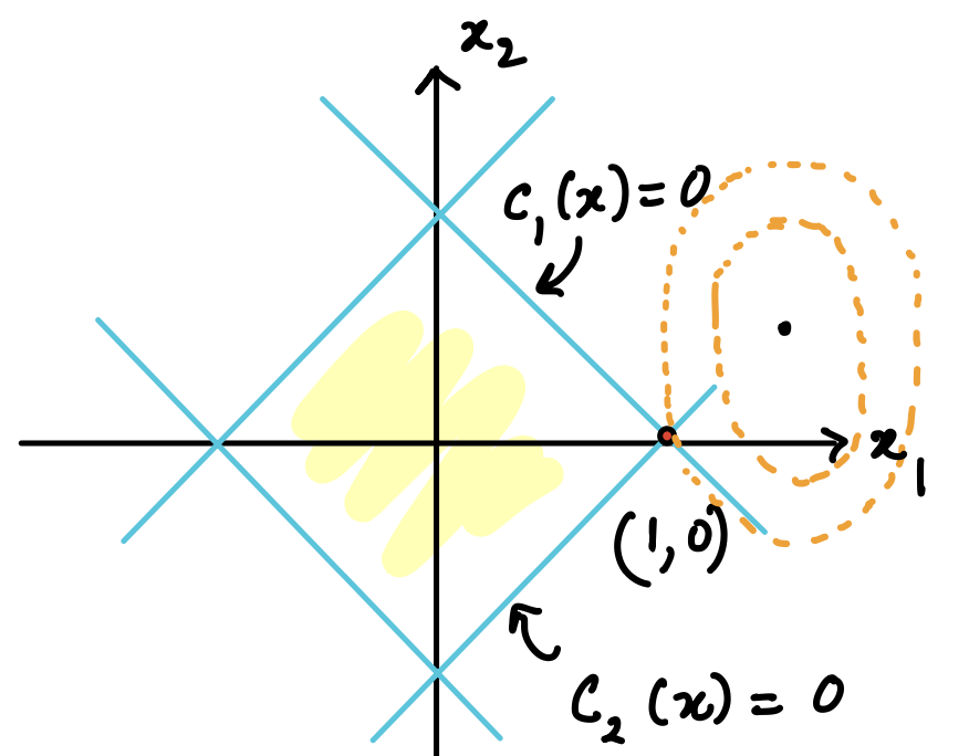
It does seem as though the optimal point might be at \((1,0)\), which is feasible and at the intersection of two of the constraints. So, we can use the recently derived theorem and check whether or not it is an optimal point.
Let’s proceed systematically:
-
Let’s list out the constraints as \(c_1(x) = 1 - x-1 - x_2, \,c_2(x) = 1 - x-1 + x_2, \,c_3(x) = 1 + x-1 - x_2, \,c_4(x) = 1 + x-1 + x_2\), all of them such that \(c_i(x) \geq 0\). Clearly, all of \( f, c_i's\) are continuous and differentiable.
-
At the point under consideration, only the \(c_1, c_2\) constraints are active. We also see that the gradients of the active constraints are \( \nabla c_1 = \begin{bmatrix} -1 \\ -1 \end{bmatrix}\) and \( \nabla c_2 = \begin{bmatrix} -1 \\ 1 \end{bmatrix}\). These two vectors are linearly independent, therefore LICQ holds.
Thus, we have satisfied the "if" parts of the theorem and proceed to the implications that must hold if \((1,0)\) is an optimal point:
-
From the complementarity conditions we can infer that the corresponding Lagrange multipliers for \(c_3,c_4\) (inactive constraints) are zero.
-
The KKT theorem then tells us that: \(\nabla_x \mathcal{L}(x,\lambda) = \nabla f(x) - \lambda_1 \nabla c_1(x) - \lambda_2 \nabla c_2(x) = 0\), i.e. \(\begin{bmatrix} -1 \\ -0.5 \end{bmatrix} + \lambda_1 \begin{bmatrix} 1 \\ 1 \end{bmatrix} + \lambda_2 \begin{bmatrix} 1 \\ -1 \end{bmatrix} = 0\), which has a solution \( \lambda_1 = 0.75, \lambda_2= 0.25, \lambda_3 = 0, \lambda_4 = 0\).
-
Since the Lagrange multipliers corresponding to inequalities are all found to be non-negative, all the "then" parts of the theorem are also found to hold. Thus, we can conclude that the point \( (1,0)\) is first-order optimal. In this case, it also turns out to be the true solution (recall that KKT conditions are first order necessary, not sufficient conditions. For sufficiency, we have to go to second order conditions).