Data, Statistics and Probability

Lecture 10: Two random variables (discrete+continuous, both continuous)

Jul-Nov 2022

Iris data set

  • First used by R. A. Fisher (https://en.wikipedia.org/wiki/Ronald_Fisher)
    • "a genius who almost single-handedly created the foundations for modern statistical science"
    • "the single most important figure in 20th century statistics"
  • Iris flower
    • 3 classes of irises: 0, 1 and 2
      • 50 instances in each class
    • Data (cm)
      • sepal length (SL), sepal width (SW), petal length (PL), petal width (PW)
    • Classification
      • Given data, find class

How to probabilistically model the data?

Iris data: Exploratory analysis

Class 0
SL SW PL PW
5.1 3.5 1.4 0.2
4.9 3.0 1.4 0.2
Class 1
SL SW PL PW
7.0 3.2 4.7 1.4
6.4 3.2 4.5 1.5
Class 2
SL SW PL PW
6.3 3.3 6.0 2.5
5.8 2.7 5.1 1.9
Summary: min-max, avg, stdev
Class SL summary SW summary PL summary PW summary
0 4.3-5.8, 5.0, 0.4 2.3-4.4, 3.4, 0.4 1.0-1.9, 1.5, 0.2 0.1-0.6, 0.3, 0.1
1 4.9-7.0, 5.9, 0.5 2.0-3.4, 2.8, 0.3 3.0-5.1, 4.3, 0.5 1.0-1.8, 1.3, 0.2
2 4.9-7.9, 6.6, 0.6 2.2-3.8, 3.0, 0.3 4.5-6.9, 5.6, 0.6 1.4-2.5, 2.0, 0.3

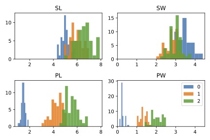
Iris data: Histograms
Iris data: How to model class and sepal length?
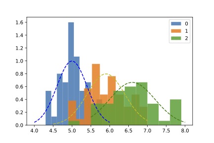
  • Density histograms of Sepal Length (SL) for all classes
    • Continuous approx: dotted lines
  • Clearly, both are jointly distributed
  • Class: discrete
  • Sepal Length (SL): continuous
    • distribution depends on class

Joint distributions: Discrete and continuous

  • : jointly distributed

  • : discrete with range and PMF

  • For each , we have a continuous random variable with density

  • : Identified as given , and denoted

  • : conditional density of given , denoted

  • Marginal density of

Example

Let . Let , and .

  • What is the marginal of ?

  • Suppose we observe to be around . What can you say about ?

Conditional probability of discrete given continuous

: jointly distributed, with PMF , conditional densities for , is the marginal density of .

  • Bayes' rule in the limit:

  • : conditional discrete random variable

  • When are and independent? is independent of .

    • and

Problems

  • Let . Let , . Find the distribution of given , , .

  • Suppose 60% of adults in the age group of 45-50 in a country are male and 40% are female. Suppose the height (in cm) of adult males in that age group in the country is Normal, and that of females is Normal. A random person is found to have a height of 155 cm. What is the chance that the person is male?

  • Let , where and are independent. What is the distribution of ? Find the distribution of .

Towards 2D probability densities

  • In 1D, it is convenient to use density function to describe "dense" random variables
    • : some interval of
    • Events collection: all unions, intersections, complements of
    • Probability function:
      • Integral defined "intuitively" as area under the curve
  • The same idea extends to 2D or even higher dimensions
    • : some 2D region of
    • Events collection: all unions, intersections, complements of
    • Probability function:
      • Integral defined "intuitively" as volume under the surface

2D histograms: (SL, SW) and (PL, PW) for Class 0
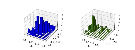
  • Count the number of falling into a rectangular bin
  • (SL, SW): Both continuous and they have a joint distribution
    • Same for (PL, PW)

Joint density in two dimensions

A function is said to be a joint density function if

  • , i.e. is non-negative
  • Technical: is piecewise continuous in each variable
  • For every joint density , there exist two jointly distributed continuous random variables and such that, for any 2D region ,

  • , also denoted , is called the joint density of and

    • supp

Example: Uniform in the unit square

Let and have joint density

  • Picture the 3D plot of the joint density
  • To compute probability, find the area of the region
  • , ,
  • ,
  • , ,

2D uniform distribution

Fix some (reasonable) region in with total area . We say that if they have the joint density

  • Rectangle:
  • Circle:
  • Multiple disjoint areas and so many other possibilities
  • For any sub-region of ,
  • Uniform distribution is a good approximation for flat histograms

Problems

  • Let , where . Sketch the support and compute , .

  • Let have joint density


Show that the above is a valid density. Find , .

Marginal density

Suppose have joint density . Then,

  • has the marginal density
  • has the marginal density
  • The joint density exactly determines both the marginal densities
  • Marginals do not determine joint density. Here are two different joint densities that result in the same marginals:
    • Uniform on unit square
    • , where

Examples

  • , where

  • , where

  • , where

  • Consider the joint density

Find the marginals.

Independence

with joint density are independent if

where and are the marginal densities.

  • Given the joint density, the marginals can be computed

  • If the joint density is the product of the marginal densities, then and are independent

  • So, if independent, the marginals determine the joint density

Examples

  • Uniform on unit square

  • , where

  • , where

  • , where

  • , where

  • Suppose , are independent random variables. Find their joint density and compute .

Conditional density

: random variables with joint density
: marginal densities

  • For such that , the conditional density of given ,

  • For such that , the conditional density of given ,

Properties of conditional density

  • Both the conditional densities are valid densities in one dimension. So, the "conditional" random variables and are well-defined.

  • Joint = Marginal times Conditional, for and such that and

  • The above is usually written as

Examples

  • Uniform on unit square

  • , where

  • , where

  • , where

  • , where

  • Consider the joint density
    Find the conditionals.

2D Jointly Gaussian


, , 2D standard normal: ,

Marginally Gaussian, but not Jointly Gaussian

  • Marginals are

  • Joint PDF is not that of 2D jointly Gaussian

  • Any others?