In this module, based off Chapter 2 of NW, we uncover the basic principles of unconstrained optimization while restricting ourselves to smooth functions.
Identifying local minima
We start with some definitions of minima. A point \(x^*\) is a:
-
global minimizer if \(f(x^*) \leq f(x) \, \forall x\in\) dom \(f\),
-
local minimizer if \(f(x^*) \leq f(x) \, \forall x\in \mathcal{N}\), where \(\mathcal{N}\) is a neighbourhood of \(x\). Such a point can further be classified as weak or strong depending on the inequality being weak or strong.
As we will find out later, when \(f\) is convex, any local minimizer is also a global minimizer. However, real world problems are often not convex and for such functions it is difficult to find global minimizers, as most approaches get trapped in local minima.
Taylor’s theorem
The central result from calculus used for deriving first and second order necessary and sufficient conditions for identifying local minima is the Taylor’s theorem. Assume that \(f: \mathbb{R}^n \to \mathbb{R}\) and that \(x,p\in\mathbb{R}^n\) and \(t \in (0,1)\). We have:
-
For a continuous differentiable function, \(f(x+p) = f(x) + \nabla f(x+tp)^T p\),
-
For a twice continuously differentiable function, \(f(x+p) = f(x) + \nabla f(x)^T p + \frac{1}{2} p^T \nabla^2f(x+tp)p\).
The above expressions can be interpreted as Taylor series + remainder term, which is why the last terms contain derivative evaluations at a point \(x+tp\) which lies in between \(x,p\). The proof is standard in Calculus texts and is omitted; interested readers may look here at the proof for a function of a single variable, and here for a discussion of the multi-variable case.
First order conditions
If \(x^*\) is a local minimizer and \(f\) is continuously differentiable in an open neighbourhood of \(x^*\), then \(\nabla f(x^*) =0\).
Proof
This is easily proved by contradiction. Assume that \(x^*\) is a minimizer but \(\nabla f(x^*)\neq 0\). Construct a new function \(g(t)=p^T \nabla f(x^*+tp)\). We are free to choose any \(p\) we want, so we choose \(p=-\nabla f(x^*)\). Clearly, \(g(t)\) is a scalar function with \(g(0)=-\|\nabla f(x^*)\|^2 < 0\) (as per our assumption). Since \(g(0)<0\) and \(g\) is a continuous function, there must be some (small) neighbourhood of \(0\) where \(g(t)<0\), i.e. \(0<t<T\). In other words, \(g(t) = p^T \nabla f(x^*+tp) < 0\) for \(0<t<T\).
Going back to the first order Taylor theorem, \(f(x^*+Tp) = f(x^*) + \nabla f(x^*+tp)^T p\), for \(t<T\), we see due to the second term on the RHS, \(f(x^*+tp) < f(x^*)\), i.e. \(x^*\) is not a minimizer, and so we have a contradiction.
The point \(x^*\) is called a stationary point if \(\nabla f(x^*) = 0\).
Second order conditions
If \(x^*\) is a local minimizer and \(\nabla^2 f\) exists and is continuous in an open neighbourhood of \(x^*\), then \(\nabla f(x^*) =0\) and \(\nabla^2 f(x^*)\) is positive semidefinite.
If \(\nabla^2 f\) is continuous in an open neighbourhood of \(x^*\) and both \(\nabla f(x^*) =0\) and \(\nabla^2 f(x^*)\) is positive definite, then \(x^*\) is a strict local minimizer of \(f\).
When \(f\) is convex, any local minimizer is a global minimizer. Additionally, when \(f\) is differentiable, any stationary point is a global minimizer.
Overview of algorithms
All optimization algorithms feature a similar approach — start with an initial guess, \(x_0\), and make a sequence of iterates, \(\{x_k\}\), to arrive at the optimal solution, \(x^*\). Broadly, two strategies are possible in going from an iterate \(x_k\) to the next \(x_{k+1}\) — line search and trust region approaches.
Line search
Here, we choose a direction \(p_k\) and search along this direction for a new iterate that has a smaller function value than \(f(x_k)\), i.e. find the length \(\alpha\) to be walked from \(x_k\) in the direction \(p_k\). Of course, the search directions and step lengths may alter between iterations. The optimization procedure considered is:
\( \{\alpha^*,p_k^*\} = \underset{\alpha,p_k}{\text{argmin}}\, f(x_k+\alpha p_k)\),
leading to \(x_{k+1} = x_k + \alpha^* p_k^*\).
Broadly speaking, there are 4 families of methods that are important in line search methods, depending on the choice of the update direction, \(p_k\). These are (details will be covered in subsequent Sections):
-
Steepest descent methods — Here \(p_k\) is chosen to be the direction in which \(f\) decreases the most, i.e. \(p_k = -\nabla f_k\).
-
Newton methods — Here second order information is used to infer a descent direction. In particular, if the Hessian, \(\nabla^2 f_k\), is positive definite, then \(p_k = - (\nabla^2 f_k)^{-1} \nabla f_k\). These methods offer faster (quadratic) convergence at a higher computational cost.
-
Quasi-Newton methods — These use approximations, \(B_k\), of the Hessian that are cheaper to compute and are typically faster than steepest descent methods. Moreover, they allow incremental computations between iterations, i.e. \(B_{k+1}\) is computed from \(B_k\).
-
Conjugate gradient methods — These use a series of descent directions that are conjugate to each other w.r.t. a system matrix. The directions take the form \(p_k = -\nabla f(x_k) + \beta_k p_{k-1}\). While these methods are not as fast as Newton or quasi-Newton methods, they do not require storage of matrices — thus making them attractive in big data computations.
The mechanism for choosing the step length \(\alpha_k\) via a line search method will be covered in a subsequent Section.
Trust region
In this approach, based on the current knowledge of \(f\) around \(x_k\), a model function \(m_k\) is constructed whose behaviour mimics that of \(f\) in a region around \(x_k\). We then search for a minimizer of \(m_k\) in a region around \(x_k\), i.e.
\( \underset{p}{\text{min}} \, m_k(x_k+p),\,\) where \(x_k+p\) lies inside the trust region.
The trust region is usually a ball defined as \(\|p\|_2 \leq \Delta\), and can be adaptively changed as the algorithm proceeds. It is common for the model to be a quadratic function like so:
\(m_k(x_k+p) = f_k + p^T \nabla f_k + \frac{1}{2} p^T B_k p,\)
where \(f_k\) and \(\nabla f_k\) are the function and gradient values at \(x_k\); thus the model agrees with \(f\) to first order at \(x_k\). Depending on the algorithm, \(B_k\) is either the Hessian or an approximation to it.
Descent directions
We summarize a few key results pertinent to the results above.
-
The steepest descent direction is given by \(-\nabla f_k\)
-
A descent direction is legitimate if it makes an angle strictly less than \(\pi/2\) with \(-\nabla f_k\)
Proof for 1 and 2
Consider a descent direction \(p_k\) and a small step length \(\epsilon\). Invoking Taylor’s theorem, we get:
\(f(x_k+\epsilon p_k) = f(x_k) + \epsilon p_k^T\nabla f_k + O(\epsilon^2)\)
If \(\epsilon\) is sufficiently small, the quadratic term may be ignored relative to the linear term. If the angle between the vectors \(p_k\) and \(\nabla f_k\) be \(\theta_k\), then:
\(p_k^T \nabla f_k = \|p_k\|\|\nabla f_k\|\cos\theta_k \)
Thus, the maximum decrease in \(f\), i.e. \(f(x_k+\epsilon p_k) - f(x_k)\), can happen when \(\theta_k = \pi\); in other words, when \(p_k \propto - \nabla f_k\). This is the direction of steepest descent.
Further, it is clear that as long as \(|\theta_k|>\pi/2\), the value of \(f\) will always decrease in this direction. Such a \(p_k\) is called a legitimate descent direction.
-
The Newton direction is given by \(- (\nabla^2 f_k)^{-1} \nabla f_k\)
Proof
Consider a second order Taylor series approximation to \(f(x_k+p)\) as:
\(f(x_k+p) \approx f_k + p^T \nabla f_k + \frac{1}{2} p^T \nabla^2 f_k p\)
Visualize the setting: we are at \(x_k\) and want to go to the next iterate \(x_k+p\), and ideally, this new iterate should be the minimizer of \(f\). If this is indeed a stationary point, then \(\nabla_p f(x_k+p) = 0\). Using the second order model and differentiating w.r.t. \(p\), this gives us: \(0 = 0 + \nabla f_k + (\nabla^2 f_k) p, \,\) (the last term evaluated by the product rule).
Re-arranging, this gives \(p = - (\nabla^2 f_k)^{-1} \nabla f_k\). Note the significance of this result — if the function to be minimized is actually a quadratic form, then one can reach the minima in one step! The price to pay is the computation of the Hessian inverse.
An example
To visualize functions and gradients consider a function \(f(x,y)=\exp(-(x-1)^2)\,sin(\pi y)\) for \(x\in[0,2],y\in[0,1] \). The figures below show the function (left) and the gradients overlaying function contours (right).
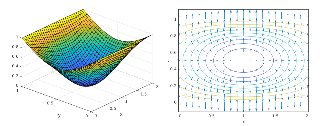
The following facts are evident:
-
The steepest descent direction always leads to a drop in the function value.
-
The steepest descent direction is not always the smartest direction to go in. For e.g. consider where the -ve gradient is pointing at \((0.1,0)\).
Matlab code
%generate function and plot it in 3D
syms x y
fs = 1 - exp(-(x-1)^2)*sin(pi*y);
fsurf(fs,[0 2 0 1])

%generate a cartesian grid to plot gradients
[X,Y] = meshgrid(0:0.1:2,0:0.1:1);
gradient(fs)
g = gradient(fs);
fx = g(1); fy = g(2);
Gx = subs(fx,{x,y},{X,Y});
Gy = subs(fy,{x,y},{X,Y});

%overlay it on contour plot
figure
fcontour(fs,[0 2 0 1])
hold on
quiver(X,Y,Gx,Gy);

%explore Hessian values at some points
H = hessian(fs);
h = subs(H,{x,y},{0.1,0});
eval(h)
eigs(eval(h)) %some eigs are negative