In this module, based off Chapter 3 of NW, we uncover the basic principles of line search methods, with a focus on the gradient (or steepest) descent method.
Step length considerations
We recall that in line search methods, once a search direction \(p_k\) is decided, the next step is to determine how much to walk in that direction, i.e. the step length \(\alpha_k\), to arrive at the next iterate:
\(x_{k+1} = x_k + \alpha_k p_k\).
We require that \(p_k\) be a descent direction, as discussed earlier (i.e. \(p_k^T \nabla f(x_k) < 0 \)), since it ensures that the function \(f\) reduces in the \(p_k\) direction (for at least small walks). This requirement on \(p_k\) is not very restrictive, and it includes several methods such as steepest descent, conjugate gradients, quasi newton, and newton methods (with some modifications).
While small walks will help reduce the value of \(f\), we should bring to mind a real world consideration: function and gradient computations, i.e. \(f(x)\) and \(\nabla f(x)\), can be expensive operations (e.g. in terms of computer time and memory). So we would like to arrive at a reasonable step length without excessive computational costs. Thus, rather than randomly trying some step lengths, or choosing very short step lengths, we need a proper strategy, which is the subject of this module.
We introduce a function of one variable (i.e. univariate):
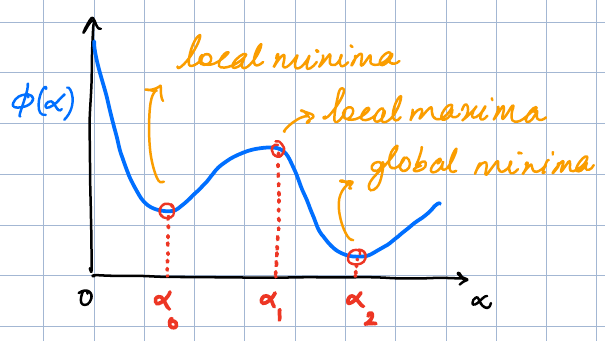
Ideally, we would like a global minimizer of \(\phi\), but this might be too ambitious an ask. For e.g. see the figure below. The blue curve represents \(\phi(\alpha)\), which is not known while we are sitting at \(\alpha = 0\) (since we have not paid the price of evaluating \(\phi(\alpha)\) for different values of \(\alpha\) so far). There are several points (e.g. \(\alpha_0,\alpha_1,\alpha_2\)) where the derivative \(\phi'(\alpha) = \frac{d \phi}{d\alpha}\) is 0 and without substantial investment in computing \(\phi,\phi'\), we don’t know which is the best \(\alpha\).
Instead, practical strategies will use an inexact line search which give an acceptable decrease in \(f\) while keeping the cost of line search itself to be moderate.
Wolfe Conditions
The Wolfe conditions form a set of inexact line search methods that comprise of the following conditions. We note one fact about our univariate function \(\phi(\alpha)\) that will be useful later. By using the chain rule, it is easy to compute the gradient w.r.t. \( \alpha\):
Sufficient decrease
The first intuitive criteria that we would like a line search method to accomplish, is a sufficient decrease in the value of the function \(f\). What would be the least expensive way of going about this? Let’s assume that at the current iterate \(x_k\), we know the function and its gradient, i.e. \(\phi(0),\phi'(0)\). Using these two pieces of information, we can form a linear approximation of the function about this point using the first order Taylor series, i.e. \(f(x_k) + \alpha \nabla f(x_k)^T p_k\), and demand that after walking a distance \(\alpha_k\), the function lie below the linear approximation. This is the red curve in figure below; the slope of the line is \(\nabla f(x_k)^T p_k\) (a negative quantity).
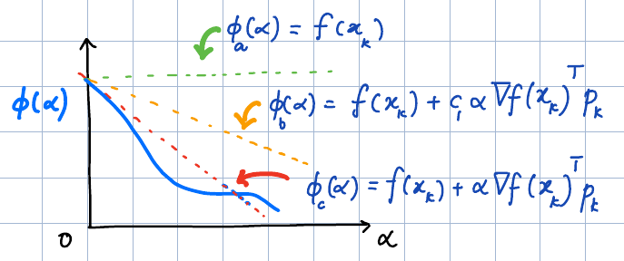
In many cases, this itself might be an ambitious ask, so we relax the condition slightly by reducing the magnitude of the slope to \(c_1\, |\nabla f(x_k)^T p_k|\), where \(c_1 \in (0,1)\). This corresponds to the orange curve in the figure above. As is graphically evident, this is a more relaxed criteria — sweeping the value of \(c_1\) from 0 to 1 sweeps us from the green to the red curve and typically, a low value \(c_1 \approx 10^{-4}\) is chosen. Formally, the condition for sufficient decrease, also called the Armijo rule, states:
Curvature condition
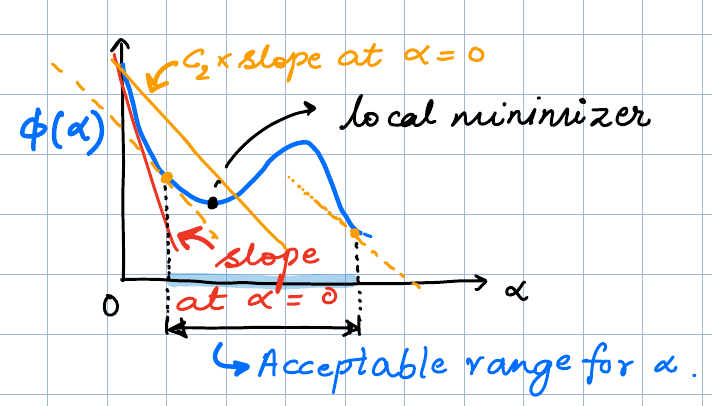
The observant reader would have noticed an insufficiency in the above criteria — very short step lengths would also pass it. To prevent this from happening, another criteria called the curvature condition is formulated. Keep in mind that our goal is to move towards a stationary point of the function \(f\), i.e. where \(\nabla f(x_k+\alpha p_k) = 0\). So, the curvature condition demands that the (magnitude of) the derivative of \(\phi(\alpha)\) at the desired \(\alpha\) be at least less than the slope of the linear approximation at \(x_k\).
In practice, the requirement is that the slope magnitude fall not just below the slope magnitude at \(x_k\), but fall below \(c_2\) times that value as seen in the figure below. Formally:
We don’t want \(c_2\) to be too small a number, else the curvature condition will become too strict, hence we bound it below by \(c_1\). Typical values of \(c_2\) are in the 0.1-0.9 range.
Note that we put negative signs in the conditions for ease of readability. Since \(p_k\) is a descent direction, we expect that \(\nabla(f(x_k)^Tp_k < 0\) and also \(\nabla(f(x_k+\alpha p_k)^T p_k < 0\) (for small values of \(\alpha\)). Thus the inequalities on both sides are positive quantities.
Strong Wolfe condition
The above remark also exposes a slight flaw in the curvature condition: it can allow a very large step length, sometimes even skipping past a stationary point, as is evident in the acceptable range for \(\alpha\) marked in the figure above.
Evidently, what has happened is that after the stationary point, we have \(\phi'(\alpha) = \nabla f(x_k + \alpha p_k) ^T p_k > 0 \). Thus the LHS of the inequality now becomes negative, while the RHS stays positive. The inequality thus remains trivially satisfied and so is of no use in preventing us from going past the stationary point.
A simple fix to this problem is called the strong Wolfe condition, which explicitly talks about the magnitudes of the derivatives, thereby preventing \(\phi'(\alpha)\) from becoming too positive. This is seen in the figure below and mathematically:
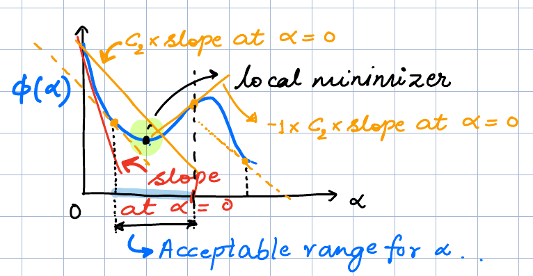
Some overshoot from a stationary point will still happen, but the extent is minimized.
Example algorithms
Backtracking line search
A very popular line search strategy involves simply working with the first condition of sufficient decrease and an intelligent way of backtracking to select an appropriate step length. The idea is to start with an initial value of \(\alpha\) (e.g. \(\alpha^{(0)}=1\)) and the sufficient decrease condition: \(f(x_k+\alpha p_k) \leq f(x_k) + c\alpha \nabla f_k^Tp_k\). If this \(\alpha^{(0)}\) is not found suitable, one simply scales it by a number \(0<\rho<1\) until the condition is satisfied, i.e. \(\alpha^{(i+1)} = \rho \alpha^{(i)}\).
Other algorithms
There is a vast amount of literature on step length selection algorithms. At one end of the spectrum, starting with an initial guess, say \(\alpha^{(0)}\) (correspondingly the value: \(\phi(\alpha^{(0)})\)), and the initial pieces of data, i.e. \(\phi(0)\) and \(\phi'(0)\), one can construct a quadratic function that satisfies the given data, and then minimize it. Refer to Sec 3.5 of NW for further details.
A popular innovation due to Barzilai and Borwein [bb] doesn’t use a linear search but instead computes the step length on information from previous iterations, for e.g. \(\alpha_k = s_{k-1}^T s_{k-1} / s_{k-1}^T y_{k-1}\), where \(s_{k-1} = x_k - x_{k-1}\) and \(y_{k-1} = \nabla(f_k) - \nabla(f_{k-1})\).
In some machine learning algorithms, a simple constant size or a decaying step size are also common.
Line Search Analysis
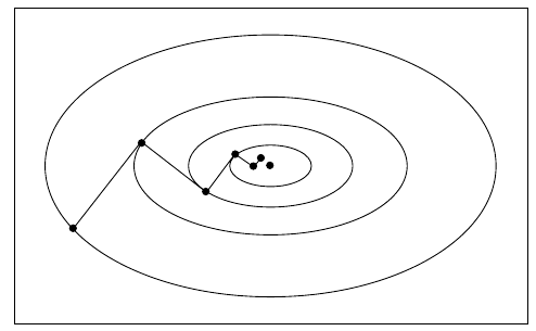
An interesting fact about exact line searches in the steepest descent method is that every step is orthogonal to the previous step.
Proof
Here we are talking about exact line searches, i.e. at the iterate \(x_k\) the step length \(\alpha_k\) is such that it minimizes \(\phi(\alpha) = f(x_k + \alpha_k p_k)\). As we’ve seen earlier, \(\phi'(\alpha) = \nabla f(x_k + \alpha_k p_k)^T p_k = \nabla f(x_{k+1})^T p_k = 0\).
With \(s_{k+1} = x_{k+1}-x_k = \alpha_k p_k\), we can compare two successive steps as \(s_{k+2}^T s_{k+1} = \alpha_{k+1}\alpha_k p_{k+1}^T p_k\). However, note that \(p_{k+1} = \nabla f(x_{k+1})\). Thus from the earlier result, we get that \(s_{k+2}^T s_{k+1} = 0\).
This fact gives us an intuition of the trajectory taken by the steepest descent iterates. For e.g. if the contours of a cost function are elongated ellipses centred at a stationary point, there will be a zig-zag motion till convergence is achieved. On the other hand, if the contours are circular, then every negative gradient direction points directly at the stationary point and convergence can be achieved in one step!
Next we take up two important issues: does the steepest descent method converge? And if so, at what rate?
Convergence
The answer is: Yes! The steepest descent method achieves global convergence in the sense that regardless of where one starts, the method converges to a stationary point. Of course, if the function is not convex, this may or may not be a minimizer.
To help us see this, we define a useful quantity: \( \cos(\theta_k) = \frac{-\nabla f_k^T p_k}{\|\nabla f_k\|\|p_k\|}. \) (Of course, in the case of the steepest descent, this angle will always be 0.)
An important theorem by Zoutendijk helps us arrive at the property of global convergence. To recall, we are considering iterations of the form \(x_{k+1} = x_k + \alpha_k p_k\), where \(p_k\) is a descent direction and \(\alpha_k\) satisfies the Wolfe conditions. The conditions of the theorem are:
-
\(f\) is bounded below, (i.e. it does not run off to \(-\infty\))
-
\(f\) is continuously differentiable in an open set \(\mathcal{N}\) that contains the level set \(\{x : f(x) \leq f(x_0)\}\) where \(x_0\) is the initialization point, and
-
the gradient is Lipschitz continuous on \(\mathcal{N}\), i.e. \(\|\nabla f(x) - \nabla f(y)\| \leq L \|x - y \|, \forall x,y \in \mathcal{N}\).
We start by invoking the curvature condition and subtracting \(\nabla f_k^T p_k\) on both sides: \( (\nabla f_{k+1} - \nabla f_k)^T p_k \geq (c_2 -1) \nabla f_k^T p_k\).
On the other hand the Lipschitz condition implies that: \( (\nabla f_{k+1} - \nabla f_k)^T p_k \leq \|\nabla f_{k+1} - \nabla f_k) \| \| p_k \| \leq L \alpha_k \| p_k \|^2 \).
Combining the above two relations gives us that: \( \alpha_k \geq \frac{c_2-1}{L} \frac{\nabla f_k^T p_k}{\|p_k\|^2} \).
We can put combine this with the first Wolfe condition to get:
\( f_{k+1} \leq f_k - c \cos^2\theta_k \|\nabla f_k \|^2\), where \(c = c_1 (1-c_2)/L\). Now it is straight forward to sum from \(0\) to \(k\) on both sides of the summation:
\( f_{k+1} \leq f_0 - c \sum_{j=0}^k \cos^2 (\theta_j) \|\nabla f_j\|^2\).
Since \(f\) is bounded from below, i.e. \(f_k\) can not \(\to -\infty\), we get that this summation is a finite quantity:
This final inequality is actually referred to as Zoutendijk’s condition. We need to just take a few more steps now. The above condition readily implies that for large \(k\), we have \(\cos^2\theta_k \|\nabla f_k\|^2 \to 0\). If we ensure in our choice of descent direction that the angle \(\theta_k\) is bounded away from 90, then \(\cos\theta_k \geq \delta > 0\). With this in place, we get that:
thus proving convergence to a stationary point.
Other proofs are also possible. For e.g. see here (Theorems 5.1 and 5.2) for proof of convergence with fixed step sizes, or for backtracking linear search.
Rate
Now that we have seen that the steepest descent method converges, we ask what rate it converges at. We will find that this rate is linear. Rather than attempting a general proof, we will prove it for a special type of objective function, one that is convex and quadratic. Further, we will limit ourselves to exact line searches. The proof sketch gives us an intuition that can be applied to more general problems.
Here is our objective function:
\(f(x) = \frac{1}{2} x^T Q x - b x\), where \(Q\) is symmetric and positive definite.
We know that for such a function, an exact line search gives the step length in closed form, leading to the steepest descent iteration being
Now, another little trick: when trying to measure convergence, we want to quantify the distance between \(x_k\) and a stationary point \(x^*\). We can try the usual norm \(\|.\|_2\), but that’s not very helpful. Instead, we introduce a new norm defined as \(\|x\|_Q = x^TQx\) (this satisfies the definition of a norm when \(Q\) is positive definite).
To see how this helps, recall that \(\nabla f_k = Q x_k - b\), and that at a stationary point \(x^*\), we will have \(Q x^* = b\). Using this definition, we can derive that: \(\frac{1}{2} \|x - x^*\|_Q^2 = f(x) - f(x^*)\), which is useful because the norm measures the difference in objective function values. With some amount of algebra, we get an important result due to Luenberger (Sec 8.2 here):
There are two immediate implications to the above result:
-
Convergence of the method is linear (also, can’t expect to do better with inexact line searches); this means to get \(f(x^{(k)}) - f(x^*) \leq \epsilon\), we need \(O(1/\epsilon)\) iterations. This holds even if we change the line search method to a fixed step size or to the backtracking line search (see here).
-
Recall that \(\kappa(Q) = \lambda_n/\lambda_1\) is the condition number of \(Q\). Thus, as the condition number worsens, the rate of convergence lowers.
The last point above can be linked to the geometric intuition conveyed by the figure above. As the condition number grows, the contours grow more elongated, and the net movement towards the minima is reduced due to the zig-zag motion. On the other hand, with \(\kappa(Q)=1\), the contours are circular and one reaches the minima in one shot.
There are other proofs of convergence available, e.g. for those approaches using backtracking line search, etc. and all of them give the same linear rate of convergence.