In this module, based off Chapter 1 (and partly 2) of NW, we discuss the broad themes in the vast subject that is optimization.
Key elements
It is the nature of nature to be efficient, to not waste. This efficiency may be thought of as another expression of evolution itself. While nature is efficient, the human mind tries to do even better (with varying degrees of success!).
When expressed in the human language of technology/engineering, this endeavour comes to be called Optimization. It is all around us, from core engineering problems to the most mundane everyday problems. As an example, consider a courier who needs to deliver packages in a residential area by spending the least amount of fuel driving, while prioritizing certain packages over others. Once the area becomes large and the number of packages many, it’s no longer possible to solve this problem by simple heuristics or rules of thumbs, and a systematic approach is needed. Enter Optimization.
Let us understand the key ideas that constitute an optimization problem:
-
Identifying an objective — the quantitative measure at the heart of the problem, typically something you want to maximize or minimize.
-
The variables — what the objective is a function of.
-
The nature of the variables — constrained or unconstrained, i.e. are the variables free to take on any values or are there restrictions.
The above elements constitute the problem model. What happens after this?
-
We proceed to find or create a suitable algorithm to solve the optimization problem. Some problems are easy to solve, for e.g. convex problems, and solving them is almost a matter of technology now, whereas other problems, such as nonlinear problems are more of an art. So, there is always a trade off between how realistic (and therefore how difficult) our problem model is and the ease with which we get a solution.
-
After the above step, we should go back and identify if we managed to find a good solution. In some cases, there are optimality conditions for checking how good a job was done. This can often give information about how to refine the problem model itself.
Next, we take a look at the different types of optimization problems that are encountered in practice.
Types of problems
Continuous v/s Discrete
As the name suggests, this refers to the nature of the optimization variables. For e.g. if the variables are real valued (i.e. the set from which the variables are drawn are uncountably infinite), it is a continuous optimization problem.
At the other end of the spectrum, if the variables are restricted to discrete values, such as integer values, we term it as a discrete optimization problem. We can even have a mix of both, and such problems are called mixed integer programming problems.
In general, the continuous optimization problems are easier since the smoothness of functions allows to say something about the behaviour of a problem in the neighbourhood of a point. However, this is not a given in discrete optimization problems — for e.g. even if two points are "nearby", there need not be any correlation between the values of the objective function at these two points. In this course we will focus on continuous optimization problems.
Constrained v/s Unconstrained
Another type of distinction can be made on the nature of the optimization variables. If they face no restrictions, we term the problem as unconstrained. On the other hand, in constrained problems there can be restrictions, such as certain equalities or inequalities that they need to obey. These restrictions can further be linear or nonlinear.
Global v/s Local optimization
It is easiest to illustrate the difference between global and local optimization by seeing the figure below . The graph is of the function \(y=|x|\sin(x)\) and let us pretend that it is the objective function of a single optimization variable \(x\).
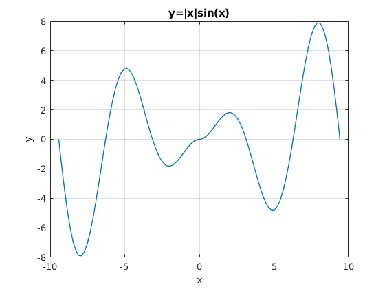
In local optimization problems, we might be interested only in finding minima in the neighbourhood of a point. For e.g. I might be interested in finding a minima for \(x\in [4,6] \). There are other such local minima in the graph. There also seems to be a global minima for \(x\in [-9,-7] \), which would be the subject of a global optimization problem.
Global optimization is in general much more difficult than local optimization because many algorithms get "stuck" in local minima (not very different from us humans getting stuck in "comfort" zones!). While this course will focus on local optimization problems, we note that many of the tools required to global optimization problems are common to local optimization problems.
Convex optimization problems have the special property that any local minima is the global minima. That said, many engineering problems need not be convex.