In this module, based off Chapter 5 of NW, we uncover the basic principles of conjugate gradient (CG) methods in their linear and nonlinear versions. Apart from NW, there is a wonderful tutorial paper written by Jonathan Shewchuk text [JS], recommended not just for the exposition on the CG method, but also as an exemplary example of technical writing.
Preliminaries
What is the problem?
The CG method is an iterative method of solving a linear system of equations of the form \(Ax = b\), where \(A\) is a symmetric positive definite matrix.
There is an equivalent way of stating this problem from an optimization perspective, which is:
since it is clear that both have the same solution. While obvious, it is helpful to state the gradient expression,
where \(r\) is called the residual.
Orthogonal matrices
In order to prepare ourselves for the road ahead, it pays to recall some results about the spectral theorem and orthogonal matrices. If \(A\) is a symmetric positive definite matrix, then as per the spectral theorem we know that \(A = U \Lambda U^T\), where \(\Lambda\) is a diagonal matrix of (positive) eigenvalues, and \(U = [u_1 \ldots u_n] \) is an orthogonal matrix with columns as eigenvectors. For an orthogonal matrix these properties hold:
-
Its inverse is given by its transpose: \(U^{-1} = U^T\),
-
Multiplication preserves length: \(\|Uq\| = \|q\|\),
-
Multiplication preserves angles: \((Uq,Ut) = (q,t)\).
Visualizing quadratic forms
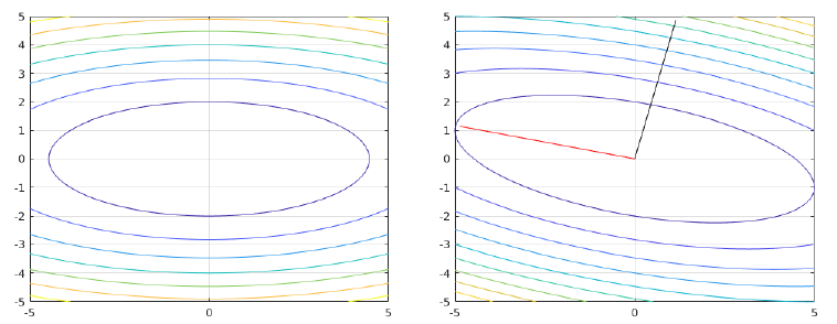
It is useful to visualize expressions of the form \(q(x) = x^T A x\). First consider the case where \(A\) is a diagonal matrix. In such a case the simplification is easy, \(q(x) = \sum_i A_{ii} x_i^2\), which is the equation of \(n\)-dimensional ellipsoid with axis coincident with the coordinate axis.
Now let’s consider what happens when \(A\) is not diagonal. Invoking the spectral theorem, we can write \(q(x) = x^T U\Lambda U^Tx = y^T \Lambda y = \sum_i \lambda_i y_i^2\), where the vector \(y=U^Tx\) can be simply viewed as a rotation of \(x\) due to the properties of the orthogonal matrix \(U\). Thus, in a coordinate system that is rotated by \(U\), we get back an \(n\)-dimensional ellipsoid. See the figure below.
Conjugacy property
We are familiar with the property of orthogonality between vectors. A related concept is that of conjugacy. We say that a set of vectors \( \{p_1,\ldots,p_l\} \) is said to be conjugate w.r.t. a symmetric positive definite matrix \(A\), if:
A remarkable property of these vectors is that they are linearly independent!
Proof
By contradiction.
Conjugate direction method
Having established all these useful results above, we get back to the problem at hand, and seek a familiar iterative method of the form \(x_{k+1} = x_k + \alpha_k p_k\), except that this time \(p_k\) need not be a descent direction. Instead, we require that:
-
The set of vectors \(\{p_1,p_2,\ldots,p_k\}\) is conjugate w.r.t. \(A\), and
-
The step length \(\alpha_k\) is an exact minimizer of the quadratic form \(\phi(x)\), i.e. \(\alpha_k = - \frac{r_k^Tp_k}{p_k^TA p_k}\) (we have pointed out earlier that the residual vector is \(r_k = A x_k - b\)).
We now state an important result:
For any \(x_0\in \mathbb{R}^n\), the sequence \(\{x_k\}\) generated as per the above specifications on \(p_k,\alpha_k\) converges to the solution \(x^*\) of the system \(Ax = b\) in at most \(n\) steps.
Proof
The proof involves straight forward linear algebra. Let us assume w.l.o.g that \(k \leq n\). Since we have earlier proved that the conjugate directions \(p_0,\ldots,p_{n-1}\) are linearly independent, it follows that we can express any vector in the \(\mathbb{R}^n\) using them as a basis; \(x^* - x_0 = \sigma_0 p_0 + \ldots \sigma_{n-1} p_{n-1}\). Using the conjugacy property, this leads to \( \sigma_k = p_k^T A (x^* - x_0)/p_k^TAp_k\).
Next, we expand the iteration expression to get: \(x_{k} - x_0 = \alpha_0 p_0 + \alpha_1 p_1 + \ldots + \alpha_{k-1} p_{k-1}\). Note — This also looks like a linear combination of basis vectors \(\{p_i\}\)! So the question is: are the \(\sigma\)'s and \(\alpha\)'s related?
Take the latter expression and premultiply \(p_k^TA\) to get \(p^T_kA(x_k - x_0) = 0\). Getting back to the numerator of the \(\sigma\) expression, we note: \( p_k^TA(x^*-x_0) = p_k^TA(x^*-x_k+x_k-x_0) = p_k^TA(x^*-x_k) = p_k^T(b- A x_k) = -p_k^T r_k\). Evidently, \(\sigma_k = \alpha_k\).
Thus, every walk along each conjugate direction is optimal and can get us to the correct solution in a maximum of \(n\) moves.
How can we visualize the above result? First consider the case when \(A\) is diagonal; in such a case the coordinate directions \(e_i\) are themselves the conjugate directions (check \(e_i^TAe_j =0\) for \(i\neq j\)), so every step is a walk along one of the coordinate directions.
Now consider the general case where \(A\) is not diagonal. Let us pull all the conjugate directions into a matrix defined like so: \(P = [p_0 \ldots p_{n-1}] \). In this case, the matrix \(D = P^TAP\) is diagonal by the conjugacy property; as a result we can rewrite the quadratic term \(x^TAx\) as \((x^T (P^{T})^{-1} P^T A P (P^{-1}x)\). With \(y=P^{-1}x\), and the commutative property of {transpose/inverse}, the quadratic term becomes: \( y^T D y\). Thus, we can visualize the conjugate direction method as steps along the coordinate directions in \(y-\) space. Recall that \(x = Py\). Thus, a step in a given coordinate direction in the \(y-\) space is actually a step along a particular \(p_i\) in the \(x-\) space.
The above discussion suggests an important intuition: once an optimal step is taken along one of the conjugate directions, that particular direction need not be revisited. This is another way of interpreting the above result’s "at most \(n\) steps" part. This intuition is formalized in the following important result:
Say that the conjugate direction method is used to generated a sequence \(\{x_k\}\) starting from \(x_0\) in order to minimize \(\phi(x)\); then these two results hold:
-
The residual at step \(k\) is orthogonal to all previous conjugate directions, i.e. \(r_k^T p_i = 0\) for \(i \in [0,k-1]\),
-
In the affine space: \(\{x|x=x_0 + \text{span}\{p_0,\ldots,p_{k-1}\}\}\), \(x_k\) is the minimizer of our functional \(\phi(x)\).
Proof
Recall that \( r(x) = Ax-b = \nabla \phi(x)\).
Consider some point \(\hat{x}\) that belongs to the described affine set, i.e. \(\hat{x} = x_0 + \sum_{i=0}^{k-1} \sigma_i p_i\). If we want to find the \(\sigma\)'s such that this point is a minimizer of \(\phi(x)\) within this affine set, we would need that: \( \frac{\partial\phi(x_0 + \sum_i \sigma_i p_i)}{\partial \sigma_i} = 0\) for \(i \in [0,k-1]\), i.e. \(k\) such equations. Since \(\phi\) has a pos. def. Hessian, it is strictly convex and thus the minimizer is unique. Using the multivariable chain rule gives us:
\(\frac{\partial \phi}{\partial \sigma_i} = \nabla \phi(x_0 + \sum_i \sigma_i p_i)^T p_i = 0\) for \(i \in [0,k-1]\). Recalling the definition of \(r(x)\), this gives us \(r(\hat{x})^T p_i = 0\) for \(i \in [0,k-1]\).
Note the iff implications of the above derivation:
-
If \(\hat{x}\) is a minimizer then \(r(\hat{x})^T p_i = 0\) for \(i \in [0,k-1]\).
-
As well as, if \(r(\hat{x})^T p_i = 0\) for \(i \in [0,k-1]\), then \( \frac{\partial\phi(x_0 + \sum_i \sigma_i p_i)}{\partial \sigma_i} = 0\) for \(i \in [0,k-1]\), which implies that the point \(x_0 + \sum_i \sigma_i p_i\) is a stationary point, which implies that it minimizes \(\phi\).
The first result can be proved by induction. For the case \(k=1\), since \(\alpha_0\) is the step length for exact minimization, \(x_1 = x_0 + \alpha_0 p_0\) minimizes \(\phi\) along \(p_0\). This implies that \(\frac{d\phi(x_0+\alpha p_0)}{d\alpha} = \nabla \phi(x_0+\alpha p_0)^Tp_0 = r(x_1)^T p_0\).
The induction hypothesis then assumes the result for \(k-1\) and uses it to prove it for \(k\). From the iff condition proved earlier, it follows that \(x_k\) is a minimizer of \(\phi\) over the given affine set.
Let us now prove the result by induction. The hypothesis for \(k-1\) says that \(r_{k-1}^Tp_i = 0\) for \(i\in[0,k-2]\). Since \(r_k = Ax_k -b\), we get \(r_{k+1} - r_k = A(x_{k+1} - x_k)\). But the term in parenthesis is just \(\alpha_k p_k\), thus \(r_{k+1} = r_k + \alpha_k A p_k\). It follows that \(r_{k} = r_{k-1} + \alpha_{k-1} A p_{k-1}\).
Now, left multiply by \(p_i\) for \(i\in[0,k-2]\): \(p_i^T r_k = p_i^T r_{k-1} + \alpha_{k-1} p_i^T A p_{k-1} = 0\). This happened because the first term on the RHS is 0 due to the induction hypothesis and the second term on the RHS is 0 due to conjugacy of \(p_i\). All that remains is to show the result for \(i=k-1\).
Left multiplying by \(p_{k-1}^T\) we get: \(p_{k-1}^Tr_k = p_{k-1}^T r_{k-1} + \alpha_{k-1} p_{k-1}^T A p_{k-1} =0 \) by the definition of \(\alpha_{k-1}\).
Thus the induction is complete since we have shown \(r_k^T p_i=0\) for \(i\in[0,k-1]\).
To summarize, while Theorem 1 gave us a general idea of convergence to the solution in at most \(n\) steps, Theorem 2 tells us properties of the residual and of solution optimality at intermediate steps.
Choice of directions
So far we have not made the choice of conjugate directions specific. There are many ways to arrive at a set of such directions, the obvious first two choices being:
-
The set of eigenvectors of \(A\). Since the eigenvectors of a positive definite matrix are orthogonal, they satisfy the conjugacy property w.r.t. \(A\).
-
Starting with any set of linearly independent vectors, the Gram-Schmidt process can be modified to output conjugate, rather than orthogonal, vectors.
However, both the methods above have a large computational cost, which becomes prohibitive for large problems (complexity \(O(n^3)\)). This observation motivates the conjugate gradient method, which we see next.
Conjugate gradient method
The power of the conjugate gradient (CG) method comes from how the conjugate directions are chosen, in particular on their low computational cost: a new direction \(p_k\) can be generated using only the previous direction, \(p_{k-1}\), and the steepest descent direction, \(-r_k\) (recall that \(r_k = Ax_k-b_k = \nabla\phi(x_k)\)). In contrast to the other directions mentioned earlier, there is no requirement of solving a system of equations. Specifically,
-
The quantity \(\beta_k\) is easy to compute by using the conjugacy property: premultiplying the above equation appropriately, we get that: \(\beta_k = (r_k^TAp_{k-1})/(p_{k-1}^TAp_{k-1})\).
-
The initial direction \(p_0\) is chosen to be the steepest descent direction at \(x_0\).
-
At each iteration, a new conjugate direction is generated, and a step length equal to \(\alpha_k = -(r_k^Tp_k)/(p_k^TAp_k)\) (as computed earlier) is taken as per: \(x_{k+1} = x_k + \alpha_k p_k\).
Practical form
The CG method can be put into a compact form as follows. Since \(r_k = Ax_k -b\), we get \(r_{k+1} - r_k = A(x_{k+1} - x_k)\). But the term in parenthesis is just \(\alpha_k p_k\), thus \(r_{k+1} = r_k + \alpha_k A p_k\). With some more algebra, we arrive at the the following simplifications:
-
\(\alpha_k = \frac{r_k^Tr_k}{p_k^TAp_k}\), and
-
\(\beta_{k+1} = \frac{r_{k+1}^Tr_{k+1}}{r_k^Tr_k^T}\).
While the above may seem like just more algebra, it reveals the power of the CG method:
-
To compute \(p_k\), we need to know \(r_k,r_{k-1}\) and \(p_{k-1}\).
-
Next, to compute \(x_{k+1}\), we additionally need to know \(p_k\).
Thus, at any given iteration \(k\), we only need to store the directions and residuals of iterations \(k\) and \(k-1\) in order to compute the next iterate \(x_{k+1}\). Apart from computing inner products, the major computational load is the computation of \(Ap_k\). Note that at no point is the explicit storage of the matrix \(A\) required — all we need is the matrix-vector product, and this is the key of the usage of the CG method for large scale problems.
Some properties
So far we have given a prescription for computing the directions \(p_k\) at each iteration, but we haven’t actually shown how these directions are conjugate w.r.t. \(A\).
At iteration \(k\) of the CG, these two results hold:
-
\(p_k^TAp_i = 0\), for \(i\in[0,k-1]\),
-
\(r_k^T r_i = 0\), for \(i\in[0,k-1]\).
Thus, the sequence of iterates \(\{x_k\}\) converges to the optimal solution in at most \(n\) steps.
Proof
Refer to the text, Theorem 5.3 of NW
Rate of convergence
We state without proof that the CG method has a linear rate of convergence. Detailed proofs can be found in Luenberger. Depending on how much information is available about the spectrum of \(A\), two results concerning the rate of convergence can be used. Assume that \(\|\cdot\|_A\) denotes the \(A\)-norm, and that the eigenvalues of \(A\) are \(\lambda_1 \leq \lambda_2 \ldots \lambda_n\), which gives the condition number as \(\kappa(A) = \lambda_n/\lambda_1\). Then, at iteration \(k\):
-
if all eigenvalues are known: \(\|x_{k+1}-x^*\|_A \leq \frac{\lambda_{n-k} - \lambda_1}{\lambda_{n-k} + \lambda_1} \, \|x_0-x^*\|_A\),
-
or, the following more conservative bound when only \(\kappa\) is known: \(\|x_{k+1}-x^*\|_A \leq 2 (\frac{\sqrt{\kappa} - 1}{\sqrt{\kappa} + 1})^k \, \|x_0-x^*\|_A\).
Several observations can be made:
-
If the eigenvalues are clustered, e.g. if there are only \(r\) distinct eigenvalues, then the CG iterations will terminate at or near the true solution within \(r\) steps.
-
Compared to the rate of convergence of the steepest descent method, the convergence is expected to be faster due to the dependence on \(\sqrt{\kappa}\), rather than \(\kappa\).
Programming
For getting more familiarity with the CG method and how it compares with the steepest descent method, click here to see a MATLAB live script showing both methods and their relative performance (raw code here). You can also study the impact of the eigenvalue distribution on the convergence of the methods. In particular, you can see that when the eigenvalues are clustered, then the CG method convergences in as many steps as the number of eigenvalue clusters — a property not shown by the SD method.
Preconditioning
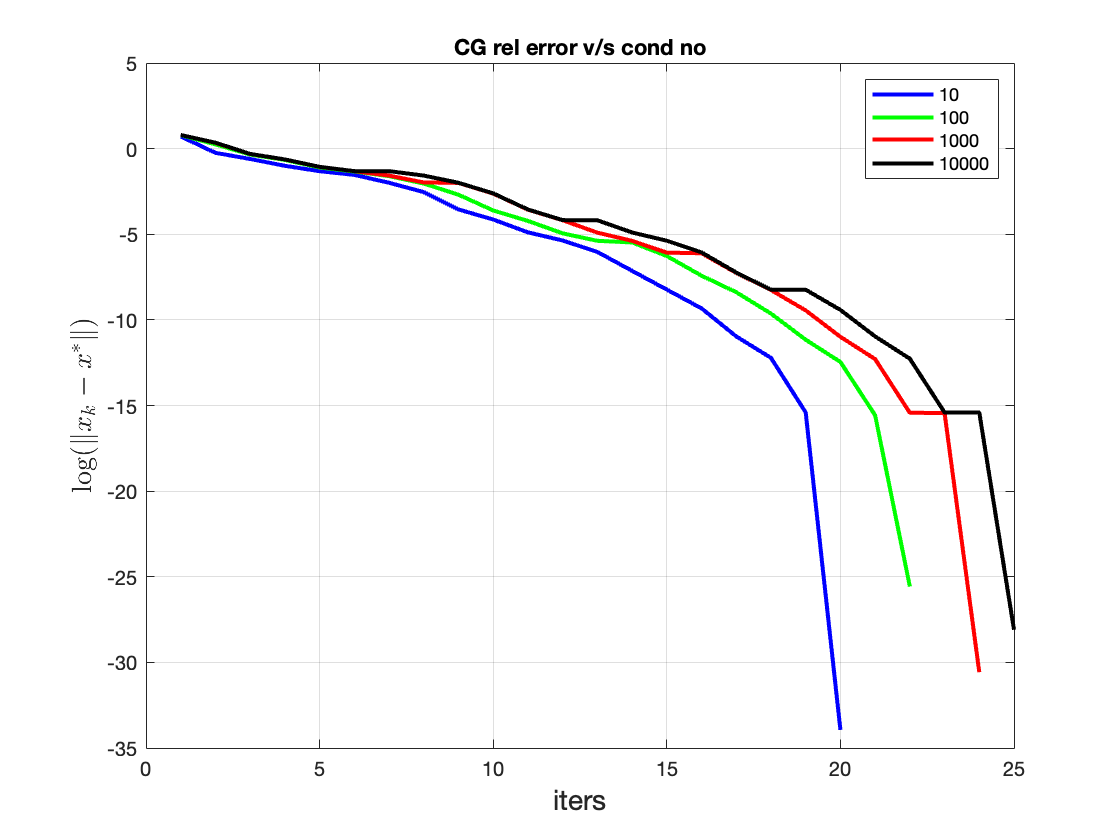
While the above description is fine to get started with "vanilla" CG, in practice it is found to be quite slow. Slow in the sense that the error diminishes slowly with iteration number, particularly if the condition number is high — this can be studied in the Figure below. Observe how, for a given number of iterations, the error is lower if the condition number is lower. Equivalently, how for a given value of error, the number of iterations required is higher if the condition number is higher (you can play with the code here).
Now let us see if convergence of the CG method can be accelerated by any method. Of course, there is no free lunch, and some computational effort will have to be budgeted for this (a bit like paying more money for faster service)! Since it is the eigen spectrum at the heart of the rate of convergence, it stands to reason that modifying it in some way holds the key to acceleration.
In order to do this, let us recall our function, \(\phi(x) = 0.5 x^TAx - b^Tx\), and insert the identity \(I = C^{-1}C\) everywhere we see \(x\). This gives us: \( \phi(x) = 0.5 x^T C^T C^{-T} A C^{-1}C x - b^T C^{-1}C x\). From here, gather a new variable as \(\hat{x} = Cx\) to get:
So, instead of worrying about the spectrum of \(A\), I need to look at the spectrum of \(C^{-T}AC^{-1}\), and the hope is that by a clever choice of \(C\), I might get better convergence. This clever choice can lead towards a clustering of eigenvalues (harder) or towards a lowering of condition number (easier).
Let us see how the algorithm works out now.
-
A naive way would be to call \(\hat{A}=C^{-T}AC^{-1}\) and \(\hat{b}=C^{-T}b\) and solve the problem \(\hat{A}\hat{x}=\hat{b}\) in the usual CG way, and to finally write \(x = C^{-1}\hat{x}\). Not surprisingly, this way is not very efficient (bad idea to be inverting matrices), so let’s see if we can perform a more invasive procedure in the hope for efficiency.
-
To motivate the more efficient way, recall that minimizing the quadratic functional is equivalent to minimizing \(Ax=b\). Now \(A\) has a bad condition number so let us pre-multiply it by a matrix product, \(CC^T\), where \(C\) is invertible. We get: \(CC^TA x = CC^Tb\). Rearranging this, we get: \(C^T A x = C^Tb\), and inserting \(CC^{-1}\) before \(x\), we get: \((C^TAC)\hat{x} = \hat{b}\), where \(x = C^{-1}\hat{x}\). Since \(\hat{A} = C^TAC\) is still sym. pos. def., the usual CG method continues to apply. Further algebra will allow us to work in the usual \(A,x,b\) system, rather than the \(\hat{A},\hat{x},\hat{b}\) system so that the number of change we need to make to our "vanilla" CG method are minimal. These are summarized below (the algebra can be seen in the class scribes):
-
initial parameters : \(p_0 = -y_0\), \(r_0 = A x_0 - b\)
-
one extra variable \(y\), defined as \(y_k = M^{-1}r_k\), where \(M^{-1} = CC^T\)
-
step length : \(\hat{\alpha}_k = \frac{r_k^T y_k}{p_k^TAp_k}\)
-
residual : \(r_{k+1} = r_k + \hat{\alpha}_k A p_k\)
-
beta parameter : \(\hat{\beta}_k = \frac{r_{k+1}^T y_{k+1} }{r_k^Ty_k}\)
-
direction update : \(p_k = -y_k +\hat{\beta}_k p_{k-1}\)
-
actual update : \(x_{k+1} = x_k + \hat{\alpha}_k p_k\)
-
A popular chocie of a preconditioner comes from the incomplete Cholesky decomposition of \(A\). Beyond this, the subject of preconditioners is vast and will not be covered further in this space.
Nonlinear CG method
In the introduction to the CG method, we had shown that solving the system \(Ax=b\) was equivalent to minimizing a convex quadratic functional. A natural extension is to ask if the CG method can be used to minimize general convex functions, or even nonlinear functions? The answer of course, is yes. The subject of optimization of nonlinear functions using the CG method is vast.
Fletcher Reeves
This being a first course on Optimization, we will discuss only the most basic nonlinear adaptation, discovered by Fletcher and Reeves. There exist many more variants, each with different features, that can be explored more in depth (for e.g. Sec 5.2 of NW).
As it turns out, we need to make only two changes to the vanilla CG method (a word on convention: earlier, we used the symbol \(\phi\) to refer to the convex quadratic function; to avoid any confusion going ahead, we will refer to the general function by \(f\))
-
Step length — since we can no longer expect an easy expression for the exact step length, a line search that identifies the minimum of the function \(f\) along a direction \(p_k\) is required.
-
Residual — earlier we had \(r(x) = Ax-b\). But recall that this was also \(=\nabla \phi(x)\). Thus, we generalize \(r(x) = \nabla f(x)\).
The resulting algorithm is just like the original approach, with these specifics:
-
The starting direction: \(p_0 = -\nabla f_0\)
-
The \(\beta\) update: \(\beta_{k+1} = \frac{\nabla f^T_{k+1} \nabla f_{k+1}}{\nabla f_k^T \nabla f_k}\)
-
The direction update: \(p_{k+1} = -\nabla f_{k+1} + \beta_{k+1}p_k\)
The appeal of this approach for nonlinear functions is high because it requires only the evaluation of the function and its gradient; further there is no storage of any matrices and only a few vectors need to be stored.
Some care needs to be taken regarding the choice of step length. Since there is no matrix "\(A\)" now, there aren’t any "conjugate directions" to talk about. Thus, we need to rely on making sure that \(p_k\) is a legitimate descent direction. To start with, let us assume that we had the luxury of exact line search. In this case, consider the expression \(\nabla f_k^T p_k\), which should be negative if the direction is a descent direction. By using the expression above, we get:
If the line search were exact, then \(\alpha_{k-1}\) would have been the exact minimizer along \(p_{k-1}\), implying that the second term on the RHS is 0. Thus, the overall expression is less than zero, therefore \(p_k\) is a descent direction. This raises the possibility that an inexact line search can cause the second term on the RHS to be large enough such that \(\nabla f_k^T p_k > 0\), and we would actually begin ascending. We state without proof, the fix for this situation: if we impose the strong Wolfe conditions with \(0<c_1<c_2<0.5)\), then it can be shown that the resulting directions are all descent directions.
We make one final note, common to many nonlinear CG variants. It can happen that at some iteration the direction \(p_k\) is "bad" (in that it is nearly orthogonal to the steepest descent direction), and the step length is too short. In such a situation, it can be shown that the directions do not change very much, i.e. \(p_{k+1} \approx p_k\), and the algorithm doesn’t make much progress. In such situations, it is preferable to set \(\beta = 0\) for one iteration. Doing so effectively "resets" the directions to start once again from the direction of steepest descent. The Polak-Ribiere method has this type of correction built into it, and is worth studying in detail.
References
-
[JS] Jonathan R. Shewchuk, An Introduction to the Conjugate Gradient Method Without the Agonizing Pain, 1994 link.